
- SAP Community
- Products and Technology
- Technology
- Technology Blogs by SAP
- Cross-Database Comparison with Aggregates
Technology Blogs by SAP
Learn how to extend and personalize SAP applications. Follow the SAP technology blog for insights into SAP BTP, ABAP, SAP Analytics Cloud, SAP HANA, and more.
Turn on suggestions
Auto-suggest helps you quickly narrow down your search results by suggesting possible matches as you type.
Showing results for
thomas_niemtsch
Discoverer
Options
- Subscribe to RSS Feed
- Mark as New
- Mark as Read
- Bookmark
- Subscribe
- Printer Friendly Page
- Report Inappropriate Content
01-05-2018
10:58 AM
Motivation
The CDC application is used to compare data sources with a complex structure or hierarchy across different systems. By doing so, you check whether the data between the source and target system is consistent, for example, whether updates in the source system have been correctly replicated to the target system. Examples of complex data sources are sales orders with several items or a master data records distributed across several tables. You can read more about CDC here.
In earlier releases, when you wanted to compare hierarchical data, such as sales order headers with their sales order items, you always had to decide on the granularity and the number of comparison keys. For instance, you could do a comparison on header level only, ignoring all sales order item information. By using both the sales order header number plus the sales order item numbers as comparison keys, the CDC would create a full extract of all order items. On one hand this allows to compare all item details, but also means an extraction and comparison of a large amount of data.
With CDC in SAP Solution Manager 7.2 you can define data models using aggregates. These allow to aggregate source data (like table rows) and only compare the result of the calculated aggregate. To stay with the sales order example, you could define a data model that compares some header information plus aggregated information of the items, e.g. a count of line items in a certain status, or even a sum of the line item values. If the source system (or to be more precise the CDC source type used) is able to generate SQL code for this, the aggregation happens directly in the source database, and only a small amount of extracted records need to be transferred to CDC, making the comparison run considerably faster.
Types of Aggregates
The following aggregate functions are supported:
- DISTINCT – Returns the values of unique records (applicable for multiple key columns)
- COUNT(DISTINCT) – Returns the number of unique records (applicable on one column only)
- COUNT(*) GROUP BY – Returns the number of records (in an independent result field)
- MIN / MAX – Returns the lowest value (minimum) / highest value (maximum) of a column, works for most data types
- AVG / SUM – Returns the arithmetic mean value (average) / sum of all values of a column, works for numeric data types only
To enable the reduction of the result set (elimination of individual data rows) due to aggregation or due to the elimination of duplicate rows from a result using DISTINCT, the SQL queries need a GROUP BY clause. This clause must contain all non-aggregated columns. Typically, these are the comparison keys. With aggregation, often you use fewer comparison keys than the source table primary keys, and then the result of the aggregate gets grouped by the remaining comparison keys. So, it is not possible to have additional classic data columns or display-only fields, because their content would have an undefined value after aggregation. Data fields or display-only fields in an aggregated format are possible of course. For this, you can select an aggregate for the field in the data model on the field details popup.
With our example of sales order items, the primary key of the item table would be the header number plus the item number. For an aggregation to a header level, we would only use the header number as comparison key. All item information gets aggregated, grouped by the header key. Possible aggregates could be the count of items, the count of distinct item units, the maximum item quantity, the sum of amounts, and so on.
In case you use aggregates that return a COUNT, the corresponding value is always an integer value, usually not matching the original data type. During the data modelling, simply do a right mouse click in the graphical editor and chose “Create COUNT GROUP BY”, to add some dummy integer field for the count value.
Example with Aggregation of items on document level
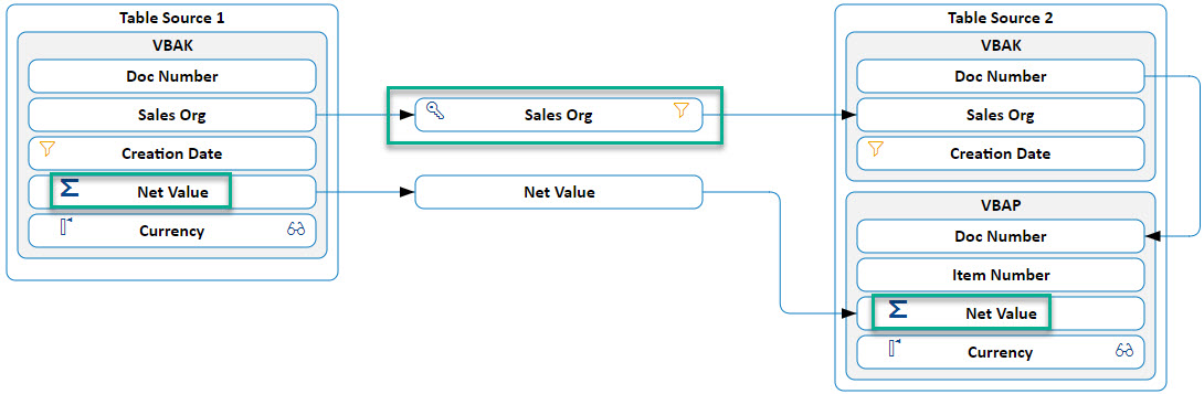
Let us look closer on the example with the SD tables VBAK (sales order header) and VBAP (sales order items). Actually, this is a system-internal comparison, where both sources are the same SAP ECC system. However, source 1 extracts the Total net value on sales order header level, which is the compared to the sum of net values on sales order item level.
In source 2, there is an aggregate of type SUM on the item net value column (VBAP-NETWR). The only comparison key is the document number (VBAK-VBELN). For source 2, containing also the joined item table VBAP, normally we would need a second comparison key for the item number (VBAP-POSNR). However, due to the aggregation of all items to the document header level, the item level becomes obsolete and thus CDC automatically generates a GROUP BY clause on the document number.
Technically speaking, we compare the transparent VBAK-NETWR field versus the aggregated SUM(VBAP-NETWR) GROUP BY VBELN.

Looking at the comparison result, we see 271 sales documents that have no item at all; no problem with that.
More interesting, there are 6 sales documents that have a real difference between their header value and the sum of item values. Two different sales organizations are affected (IWS0 and 0001).

In total, 222,698 sales documents were compared, distributed over 12 sales organizations, and that took 25 seconds. Not bad, but we can speed this up even more, knowing that the database is much faster in aggregating data than extracting data, plus transferring and comparing single document data to CDC. If only a few sales organizations are affected, why don’t first determine the affected sales organizations, and then do a detailed comparison on document level just for those?
Example with Aggregation of items to sales org level
We change our comparison model a bit. Instead of using the document number as comparison key, we even use the company code. The GROUP BY clause changes to VBAK-VKORG, and the source database now aggregates on a higher level.
For source 2 we still need the document number, but just for a join condition between header and items, where VBAP sums up the item values and aggregates it to the header’s sales organization.
As we can see in the result overview, 12 sales organizations have been compared, 10 are identical (that is the total sum of all sales document header and item net values matches perfectly), and we see exactly those two sales organizations with a difference.
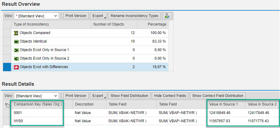
This high aggregation takes only 6 seconds for the database. Obviously, CDC has close to zero effort to just compare 12 extracted aggregated rows.
Drill-down from High-level to Low-level Aggregation
Interesting approach… we can start from a fast high-level aggregated comparison. Then we just use the identified aggregation keys (here the sales organizations) to trigger a lower-level aggregation (e.g. on sales office), and from there to single sales documents.
For our example above, the aggregate just needs 6 seconds, and then using the two identified sales organizations as variable filters in the first comparison, we just need 2 seconds to compare 1,391 sales documents (instead of 25 seconds for 222,698). In total, it needs just 8 seconds to find the 6 sales documents with value differences!

An example in the Financial area would be a chain of drill-down comparisons from company code to account to single postings.
Conclusion
As you can see, aggregates have multiple advantages, or are the prerequisite for some comparison scenarios
- They can speed up the comparison time of large data sources
- They serve as basis for defining drill-down comparisons
- They allow comparisons between non-aggregated raw data (e.g. single documents in an OLTP system) versus already aggregated data in an OLAP system
Concluding, we hope this will help you in understanding the benefit and some use-cases for applying aggregates in CDC data models. Have fun trying it out and let us know what you think!
Links
Data Consistency Management Blog: https://blogs.sap.com/2016/05/31/introduction-to-new-blog-series-on-data-consistency-management/
Data Consistency Management Wiki: http://wiki.scn.sap.com/wiki/display/SM/Data+Consistency+Management
- SAP Managed Tags:
- SAP Solution Manager,
- SOLMAN Business Process Operations
You must be a registered user to add a comment. If you've already registered, sign in. Otherwise, register and sign in.
Labels in this area
-
ABAP CDS Views - CDC (Change Data Capture)
2 -
AI
1 -
Analyze Workload Data
1 -
BTP
1 -
Business and IT Integration
2 -
Business application stu
1 -
Business Technology Platform
1 -
Business Trends
1,661 -
Business Trends
88 -
CAP
1 -
cf
1 -
Cloud Foundry
1 -
Confluent
1 -
Customer COE Basics and Fundamentals
1 -
Customer COE Latest and Greatest
3 -
Customer Data Browser app
1 -
Data Analysis Tool
1 -
data migration
1 -
data transfer
1 -
Datasphere
2 -
Event Information
1,400 -
Event Information
65 -
Expert
1 -
Expert Insights
178 -
Expert Insights
280 -
General
1 -
Google cloud
1 -
Google Next'24
1 -
Kafka
1 -
Life at SAP
784 -
Life at SAP
11 -
Migrate your Data App
1 -
MTA
1 -
Network Performance Analysis
1 -
NodeJS
1 -
PDF
1 -
POC
1 -
Product Updates
4,577 -
Product Updates
330 -
Replication Flow
1 -
RisewithSAP
1 -
SAP BTP
1 -
SAP BTP Cloud Foundry
1 -
SAP Cloud ALM
1 -
SAP Cloud Application Programming Model
1 -
SAP Datasphere
2 -
SAP S4HANA Cloud
1 -
SAP S4HANA Migration Cockpit
1 -
Technology Updates
6,886 -
Technology Updates
408 -
Workload Fluctuations
1
Related Content
- Analyze Expensive ABAP Workload in the Cloud with Work Process Sampling in Technology Blogs by SAP
- exception aggregation used in CDS view and that field is not available in SAC in Technology Q&A
- Data Flows - The Python Script Operator and why you should avoid it in Technology Blogs by Members
- Sneak Peek in to SAP Analytics Cloud release for Q2 2024 in Technology Blogs by SAP
- SAP Cloud Integration: Understanding the XML Digital Signature Standard in Technology Blogs by SAP
Top kudoed authors
| User | Count |
|---|---|
| 13 | |
| 11 | |
| 10 | |
| 9 | |
| 9 | |
| 7 | |
| 6 | |
| 5 | |
| 5 | |
| 5 |