
- SAP Community
- Products and Technology
- Technology
- Technology Blogs by SAP
- Product Cost Forecast and Simulation - how to enha...
Technology Blogs by SAP
Learn how to extend and personalize SAP applications. Follow the SAP technology blog for insights into SAP BTP, ABAP, SAP Analytics Cloud, SAP HANA, and more.
Turn on suggestions
Auto-suggest helps you quickly narrow down your search results by suggesting possible matches as you type.
Showing results for
Advisor
Options
- Subscribe to RSS Feed
- Mark as New
- Mark as Read
- Bookmark
- Subscribe
- Printer Friendly Page
- Report Inappropriate Content
11-09-2017
3:05 PM
Update February 2021:
The related SAP Business Warehouse Content has been set to "obsolete".
Please refer to SAP note 1929531.
Summary:
This blog describes a concept how to enhance the SAP HANA-optimzed Business Warehouse content Product Cost Forecast and Simulation by tariffs.
The concept bases on the detailed product cost information, that the standard data sources can provide. SAP Business Warehouse modeling and business logic are covered in detail to explain the concept.
The blog contains the following chapters:
Motivation
Product Cost Forecast and Simulation has been delivered as part of the SAP HANA-optimised BI Content for SAP Business Warehouse. Details about Product Cost Forecast and Simulation may be found in our blog or the online help.
In the standard content, the impact of conversion costs – costs resulting from manual or machine-based production steps – can be simulated on a coarse level only. However, the need to forecast and simulate these conversion costs in more detail is also a valid business case and a natural enhancement to the standard content. The conversion costs are calculated from tariffs, i.e. standard rates for activities within a company.
With the concept described in this blog, customers can implement the necessary enhancements to the standard content on their own.
Prerequisites
A comprehensive understanding of the HANA-optimized Product Forecasting and Simulation content and the technologies being used - namely SAP BW on HANA and SAP HANA including SQL scripts - is required. Ideally, the standard content has already been implemented and is up-and-running.
The blog outlines a concept and supports this with proposals of how to model SAP Business Warehouse objects and SQL code snippets. Both modelling details and code snippets are used in this document to illustrate the concept but they are not intended to be used productively.
Please read the concept thoroughly and decide, if your business needs can be covered as described. As usually it is recommended to do a proper design before starting the implementation. Other best practices like separating the development from the production and thorough testing before going into production for sure also apply here.
The concept assumes that the proposed standard SAP data sources are used (0CO_PC_PCP_20 and 0CO_PC_PCP_30). Using other data sources is feasible, but in that case the concept cannot be used out-of-the-box.
Outline of the Concept
Standard Content only uses sum of conversion costs
The data sources 0CO_PC_PCP_20 and 0CO_PC_PCP_30 can deliver the basic tariff information and the break-down of conversion costs into individual production process steps. Because the focus of the standard content is on material costs, the tariff information has so far not been used, but filtered out in the data load process. Consequently, only the content in the SAP Business Warehouse (SAP BW) and the underlying SAP HANA database need to be enhanced, no changes are required in the source system.
In general, the Product Cost Forecast and Simulation works as follows:
For each product, the required amounts of materials (“Bill of Material” or “BOM”) are known. For each material, the cost component structure and costs are known. Costs can be rolled up per cost component from raw material level to each product.
Diagram 1 shows this schematically, though real products are typically more complex.
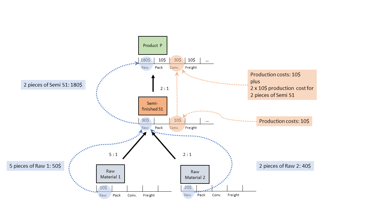
Diagram 1: Example bill of material with cost structure
In this example, the two raw materials 1 and 2 cost 10 $ and 20 $ respectively. The costs are assigned to raw material costs. No other costs exist on this level, so the other cost components are not filled.
The raw material costs roll-up to the semi-finished good S1 based on the required quantities. The production of S1 costs 10 $, that are assigned to conversion costs.
Finally, the production of product P from 2 pieces of S1 costs 10 $ plus the conversion costs of 2 pieces of S1 to add up to 30 $. The raw material costs have been rolled-up and new costs (10 $ each for packaging and freight) are considered.
The cost component information is retrieved from the data source 0CO_PC_PCP_20 and stored in the data store object (DSO) /IMO/CFS_D20. The required quantities are retrieved from the data source 0CO_PC_PCP_30 and stored in the data store object /IMO/CFS_D30.
Diagram 2 shows this schematically:

Diagram 2: Relationship of bill of material and data sources/DSOs
This is what the standard content currently covers. In the current example, the conversion costs that reflect the complete production process can be treated as lump sums.
While it is feasible to change the conversion costs in total, a differentiated view and a simulation of tariff changes are not offered. However, the data sources already deliver a break-down of the total conversion costs per material. The concept described in this paper aims to help implement a tariff-based forecast and simulation.
A breakdown of production costs brings higher precision
The total conversion costs can be broken down into several components – here manual labour and machine hours of two machines M and N.
Diagram 3 shows this:

Diagram 3: Example break-down of production costs
The production of 1 semi-finished good S1 requires (in addition to the materials) 5 minutes of manual labour and 10 minutes of machine M. The tariffs are 15,00 $ and 52,50 $ for 1 hour respectively. Similarly, the production of the product consumes 20 minutes of manual labour and 5 minutes of machine N. Taking the respective tariffs into account, this sums up to 10 $.
This break-down allows to simulate the production costs on a finer level, which gives a higher precision. And a higher precision is required, whenever the production costs play a more important role.
Assume that an increase in wages by 1 $/h has to be simulated. In the standard content, only the sum of conversion costs could be changed: The increase of 6% in wages could be used to change all conversion costs at the same time. The impact would be the same for all conversion costs. However, we see that the wages impact the conversion costs differently, namely roughly 10% for the semi-finished good S1 and 50% for the product. This distinction cannot be made in the standard content.
Remark: This is a simplification. In the standard content one could actually differentiate between semi-finished goods and products. For the sake of keeping the example easy to understand, this fact is neglected here. However, within the group of products or the group of semi-finished goods a distinction is not possible; but important for the same reason outlined here.
What needs to be done to achieve this break-down?
The concept describes two ways of dealing with tariffs, quite similar to the two ways of dealing with material costs: individual changes to one tariff and a driver-based approach to change several tariffs simultaneously.
In our case, changing the hourly wage from 15 $ to 16 $ is an individual change. Changing the machine hour tariffs for both machines M and N because of an increase of the energy costs is a driver-based approach, changing several tariffs by one driver (energy costs).
- Calculate and store tariff to material link
The data source delivers the amount of work (usually a time) and the costs per material.
The first step is to calculate the tariffs from this information: In our manual labour example, 5 min cost 1,25 $. So, the hourly tariff amounts to 15 $.
The tariffs are stored together with the individual materials. - Store “standard” or “actual” tariffs as basis for planning
Tariffs calculated in step 1 are stored in a dedicated InfoProvider without a connection to materials: This is the base line for planning. Also, these “standard” or “actual” tariffs serve as a reference when manually planning future tariffs.Remark: Test have not shown, that different tariffs can exist for the same activity but different materials or cost components. Please verify, that this assumption is valid for your source system. Tariffs have to be unique. - Store “plan” tariffs and create suitable input-ready query
The tariffs need to changeable individually. From a technical perspective, this requires them to be input-ready. - Correlate drivers to tariffs In addition, the already existing drivers (stored in data store object /IMO/CFS_D01) have to be correlated to the tariffs. This requires an InfoProvider similar to the correlation of drivers and materials.Remark: The grouping of materials and the introduction of so-called material-driver-segments is feasible, but not covered in the following text. The reader may decide to introduce a similar grouping if necessary.
- Adapt business logic
The underlying business logic has to be enhanced: The tariff-based cost changes have to be calculated and then summed up into the corresponding cost components (there could be more than one, simplified for this example).Remark: This can be done either in a dedicated SQL procedure or through enhancing existing SQLs.Once the cost components have been adjusted based on the tariff changes, the roll-up logic to calculate the total costs of a product remains unchanged. And the preparation step, that calculates how many pieces/units of a certain material are required to produce a given product (table /IMO/CFS_ITEMZTN) also remains unchanged.
- Calculate and store tariff to material link
The required changes are shown in Diagram 4:

Diagram 4: Overview of changes and enhancements
Implementation of the Concept
This chapter provides detailed information about the 5 enhancements.
Be reminded that all data models and SQL snippets are shown to explain the concept in detail. They should not be used without verification and possibly adaptations in your landscape.
The key and data fields are listed (as screen shots). Wherever possible, standard InfoObjects are used, but in certain cases new fields are introduced. It is recommended to stick to standard fields in the same way. If this is not appropriate, please make sure you also adapt any subsequent object and SQL business logic.
Calculate and store tariff to material link
Create an InfoProvider to hold the links between tariffs and the individual materials. In the prototype, the InfoProvider is called ZCFS_T_M (“Tariff to Material Link”).
Use the following fields as shown in Diagram 5:

Diagram 5: Field list “Tariff to Material Link” InfoProvider
In addition to First Planning Period and Fiscal Year Variant, there are two groups of keys that define the two business entities “Material” and “Tariff”: The yellow box contains the fields that identify the Material, the blue box contains the fields that uniquely define an activity to which a tariff is assigned. 0PLANT belongs to both groups.
In the prototype, we introduced the key figure ZCFS_TF in which the calculated tariffs are stored. The key figure is of data type “CURR” and has “0CURRENCY” as Currency.
The tariff has to be calculated based on 0AMOUNT and 0QUANTITY:
ZCFS_TF = 0AMOUNT / 0QUANTITY.
The data flow for this InfoProvider is based on the InfoSource /IMO/CFS_IS30 (Product Costing Analysis: Itemization (0CO_PC_PCP_30)).
The transformation rules can be found in Diagram 6:

Diagram 6: Transformation Rule "Tariff to Material Link"
All fields are directly assigned from the InfoSource to the InfoProvider except for:
- 0CFS_FPP: this field is sourced from a routine. Please use the same routine as the standard content. Check the transformation rules from InfoSource /IMO/CFS_IS30 to InfoSource /IMO/CFS_IS301 for details.
- 0FISCVARNT: same as for 0CFS_FPP
- ZUNIT: a dedicated characteristic has been defined which is sourced from 0UNIT
- ZCFS_TF: calculation – see above
The Filter for the data transfer process has to be set as follows: select “2” for Stufe and exclude the Item Categories “I”, “L” and “M”.
Store “standard” or “actual” tariffs as basis for planning
Create an InfoProvider to hold the standard or actual tariffs. In the prototype, the InfoProvider is called ZCFS_T_L (“Standard Tariffs”).
Use the following fields as shown in Diagram 7:

Diagram 7: Field List „Standard Tariffs” InfoProvider
Remark: The cost components have been included. This is necessary if the conversion costs are kept in more than 1 cost component. If conversion costs always refer to one single cost component, this InfoProvider may be simplified by omitting 0COSTCOMP / 0CCOMPSTRUC. The other enhancements can then be simplified accordingly.
The “Standard Tariffs” InfoProvider is filled from the “Tariff to Material Link” InfoProvider (see above). The transformation rules can be found in Diagram 8:

Diagram 8: Transformation Rule „Standard Tariffs“
All fields can just be moved from the source to the target. The routine for the field 0VERSION can be taken over from the standard content: Please check the transformation rule into DSO /IMO/CFS_D031. Make sure, that the Tariffs will not be summarized: Check that the aggregation rule for field ZCFS_TF is set to overwrite.
Store “plan” tariffs and create suitable input-ready query
Create an InfoProvider to hold the plan tariffs. In our prototype, the InfoProvider is called ZCFS_T_P (“Plan Tariffs”).
Use the InfoProvider “Standard Tariffs” as a template to create the “Plan Tariffs” as a planning enabled InfoProvider. Switch on “External SAP HANA view”.
Add the field 0FISCPER as Key field. The complete field list is shown in Diagram 9:

Diagram 9: Field List "Plan Tariffs" InfoProvider
Create a MultiProvider or Composite Provider which includes the two InfoProviders “Standard Tariffs” and “Plan Tariffs”. Include all fields of the InfoProvider “Plan Tariffs”. Identify (Assign) all field to both InfoProvider, 0FISCPER will only be mapped to “Plan Tariffs”.
Based on the MultiProvider / Composite Provider, create an Aggregation Level that contains all the fields. Create a suitable Filter and create a Planning Function of type copy to fill the InfoProvider “Plan Tariffs” as follows:

Diagram 10: Define Fields to change
Set the following fields to be changed: 0FISCPER, 0INFOPROVIDER and 0VERSION.
In the prototype, the 0CFS_FPP has been chosen to define a condition. In the copy process, the version has to be changed from “actual” to “plan” and the InfoProvider has to be changed from “Standard Tariffs” (ZCFS_T_L) to “Plan Tariffs” (ZCFS_T_P). The data has to be copied to fill the remaining fiscal periods in accordance with the setting of the planning horizon (DSO /IMO/CFS_D05).
The following example has been taken from the prototype:

Diagram 11: Copy Standard Tariffs to Plan
Based on the Aggregation Level, create an input-ready query that allows to manually adjust the plan values for the future periods. It is recommended to show the standard tariff values for reference. Refer to other input-ready query in the standard content for details.
Correlate drivers to tariffs
The cost drivers are planned based on DSO /IMO/CFS_D01 “Cost Drivers”.
The correlation of tariffs to a driver works analogously to the correlation of material groups (called “Material-Driver-Segments”, 0CFS_SEGMNT). For details, check the standard content DSO IMO/CFS_D02 “Correlation Cost Drivers”.
Adapt business logic
Based on the new InfoProviders created, the business logic needs to be adapted as follows:
- New SQL logic to calculate the changes of cost component values based on the tariffs
- Incorporate changed values in existing logic
Calculate changes based on tariffs
First, a new SQL procedure has to be created (or the new logic has to be implemented in the existing procedures). The following code snippets illustrate the logic. They need to be adjusted to fit to your system and setup and must not be used productively.
Remark: The code snippets do not use CE-functions, even though the standard content does.
In the first step, the materials and their tariffs are read in. As common in Product Cost Forecast and Simulation, in this step the tariffs are copied over (“expanded”) to all fiscal periods defined by the planning horizon.
-- Read in the CO-PC tariffs baseline

-- and expand them to the planning horizon


 join1 = select

        d0."0VERSION" as "0VERSION" ,

        t0."0CFS_FPP" ,

	t0."0FISCVARNT" ,

	d0."0FISCPER" ,

	t0."0MAT_PLANT" as "0MATERIAL" ,

	t0."0PLANT" as "0PLANT" ,

	t0."0CCOMPSTRUC" ,

	t0."0COSTCOMP" ,

	t0."0ACTTYPE" ,

	t0."0COSTCENTER" ,

	t0."0COSTELMNT" ,

	t0."0PCP_RES" ,

	t0."0COSTPOS" ,

	t0."0CO_AREA" ,

	t0."0UNIT" ,

	t0."ZUNIT" ,

	t0."0CURRENCY" ,

	sum(t0."0AMOUNT") as "0AMOUNT" ,

	sum(t0."0AMOUNTFX") as "0AMOUNTFX" ,

	sum(t0."0AMOUNTVR") as "0AMOUNTVR" ,

	sum(t0."0QUANTITY") as "0QUANTITY" ,

	sum(t0."ZCFS_TF") as "ZCFS_TF" ,

	round ( sum(t0."0QUANTITY") * sum(t0."ZCFS_TF") , 2 ) as "0AMOUNT_CHECK"


	from <new DSO “Tariff to Material Link”> as t0


	join


	(select "0VERSION" , "0CFS_FPP",

                "0FISCVARNT" , "0FISCPER"

	 from “_SYS_BIC"."system-local.bw.bw2hana.imo/CFS_D05”

	 where "0VERSION"   = :VERSION and

               "0CFS_FPP"   = :ACTPER and

               "0FISCVARNT" = :FISCVARNT

	) as d0


	on

        t0."0CFS_FPP"   = d0."0CFS_FPP" and

        t0."0FISCVARNT" = d0."0FISCVARNT"


	where t0."0CFS_FPP"   = :ACTPER and

              t0."0FISCVARNT" = :FISCVARNT


        group by d0."0VERSION" ,

                 t0."0CFS_FPP" , t0."0FISCVARNT" , d0."0FISCPER" ,

                 t0."0MAT_PLANT" , t0."0PLANT" , t0."0CCOMPSTRUC" ,

                 t0."0COSTCOMP" , t0."0ACTTYPE" , t0."0COSTCENTER" ,

                 t0."0COSTELMNT" , t0."0PCP_RES" , t0."0COSTPOS" ,

                 t0."0CO_AREA" , t0."0UNIT" , t0."ZUNIT" ,

                 t0."0CURRENCY"

;
Now, the drivers and the correlations are read in:
-- Read in the driver and their correlations

joind = select

        d."0VERSION" ,

        d."0FISCVARNT" ,

        d."0FISCPER" ,

        d."0CFS_DRIVID" ,

        d."0CURRENCY" ,

        c."0CCOMPSTRUC" ,

        c."0COSTCOMP" ,

        c."0ACTTYPE" ,

        c."0CO_AREA" ,

        c."0COSTCENTER" ,

        c."0COSTELMNT" ,

        c."0PCP_RES" ,

        sum(b."DRIV_BASE") as "DRIV_BASE" ,

        sum(d."0CFS_DRPRC") as "DRIV_PRIC" ,

        max(c."0CFS_COREL") as "COREL" ,

        case

        when sum(b."DRIV_BASE") = 0.0 or sum(b."DRIV_BASE") is null

        then 0.0 else (

        (sum(d."0CFS_DRPRC")-sum(b."DRIV_BASE"))/sum(b."DRIV_BASE")

         * max(c."0CFS_COREL")

        ) end as "FACTOR"


        from "_SYS_BIC"."system-local.bw.bw2hana.imo/CFS_D01" as d


        join


        (select "0VERSION" , "0FISCVARNT" , "0FISCPER" ,

                "0CFS_DRIVID" , "0CURRENCY" ,

                sum("0CFS_DRPRC") as "DRIV_BASE"

         from  "_SYS_BIC"."system-local.bw.bw2hana.imo/CFS_D01"

         where "0VERSION"   = :VERSION and

               "0FISCPER"   = :ACTPER and

               "0FISCVARNT" = :FISCVARNT

         group by "0VERSION" , "0FISCVARNT" , "0FISCPER" ,

                  "0CFS_DRIVID" , "0CURRENCY"

        ) as b

        on

        d."0VERSION"    = b."0VERSION" and

        d."0FISCVARNT"  = b."0FISCVARNT" and

        d."0CFS_DRIVID" = b."0CFS_DRIVID" and

        d."0CURRENCY"   = b."0CURRENCY"


        join


        (select "0VERSION" , "0CFS_DRIVID" , "0CCOMPSTRUC" ,

                "0COSTCOMP" , "0ACTTYPE" , "0CO_AREA" ,

                "0COSTCENTER" , "0COSTELMNT" , "0PCP_RES" ,

                max("0CFS_COREL") as "0CFS_COREL"

         from  <new DSO “Correlation to Drivers”>

         where "0VERSION" = :VERSION

         group by "0VERSION" , "0CFS_DRIVID" , "0CCOMPSTRUC" ,

                  "0COSTCOMP" , "0ACTTYPE" , "0CO_AREA" ,

                  "0COSTCENTER", "0COSTELMNT" , "0PCP_RES"

        ) as c

        on

        d."0VERSION"    = c."0VERSION" and

        d."0CFS_DRIVID" = c."0CFS_DRIVID"


        where d."0VERSION" = :VERSION and d."0FISCVARNT"= :FISCVARNT


        group by d."0VERSION" , d."0FISCVARNT" , d."0FISCPER" ,

                 d."0CFS_DRIVID" , d."0CURRENCY" , c."0CCOMPSTRUC" ,

                 c."0COSTCOMP" , c."0ACTTYPE" , c."0CO_AREA" ,

                 c."0COSTCENTER" , c."0COSTELMNT" , c."0PCP_RES"

;
The logic determines the driver values including the future values that may be changed as part of the simulation. The first join determines the so-called base line, namely the driver values for the first planning period. The percentage change of future value compared to base line value is calculated (“Factor”).
The second join determines the correlation between drivers and their future percentage changes on the one hand and the tariffs on the other hand.
As with the standard content (DSO /IMO/CFS_D21), it is possible to manually plan tariffs. In case manually planned values exist that are different to the baseline, these values are used.
join2 = select

        t0."0VERSION" ,

        t0."0CFS_FPP" ,

	t0."0FISCVARNT" ,

	t0."0FISCPER" ,

	t0."0MATERIAL" ,

	t0."0PLANT" ,

	t0."0CCOMPSTRUC" ,

	t0."0COSTCOMP" ,

	t0."0ACTTYPE" ,

	t0."0COSTCENTER" ,

	t0."0COSTELMNT" ,

	t0."0PCP_RES" ,

	t0."0COSTPOS" ,

	t0."0CO_AREA" ,

	t0."0UNIT" ,

	t0."ZUNIT" ,

	t0."0CURRENCY" ,

	t0."0AMOUNT" ,

	t0."0AMOUNTFX" ,

	t0."0AMOUNTVR" ,

	t0."0QUANTITY" ,

	t0."ZCFS_TF" ,

	t0."0AMOUNT_CHECK" ,

	tp."ZCFS_TF_PLAN_MANUAL" ,

	t0."ZCFS_TF" * td."FACTOR" as "ZCFS_TF_PLAN_DRIV" ,


	case when  tp."ZCFS_TF_PLAN_MANUAL" = 0 or

                   tp."ZCFS_TF_PLAN_MANUAL" is null or

                   t0."ZCFS_TF" = tp."ZCFS_TF_PLAN_MANUAL"

	then

		case when  ( t0."ZCFS_TF" * td."FACTOR" ) is null

		then round ( t0."0QUANTITY" * t0."ZCFS_TF" , 2 )

		else round ( t0."0QUANTITY" * t0."ZCFS_TF"

                             * td."FACTOR" , 2 ) end


	else round ( t0."0QUANTITY" * tp."ZCFS_TF_PLAN_MANUAL" , 2 )

	end  as "0AMOUNT_PLAN"


	from :join1 as t0


	left join


	(select "0VERSION" , "0CFS_FPP" , "0FISCVARNT" ,

                "0FISCPER" , "0CCOMPSTRUC" , "0COSTCOMP" ,

                "0ACTTYPE" , "0COSTCENTER" , "0COSTELMNT" ,

                "0PCP_RES" , "0CO_AREA" , "0PLANT" ,

                "0CURRENCY" , "ZUNIT" ,

                max("ZCFS_TF") as "ZCFS_TF_PLAN_MANUAL"

	 from <new DSO “Plan Tariffs”>

	 where "0CFS_FPP"   = :ACTPER and

               "0FISCVARNT" = :FISCVARNT and

               "0VERSION"   = :VERSION

         group by "0VERSION" ,

                  "0CFS_FPP" , "0FISCVARNT" , "0FISCPER" ,

                  "0CCOMPSTRUC" , "0COSTCOMP" , "0ACTTYPE" ,

                  "0COSTCENTER" ,  "0COSTELMNT" , "0PCP_RES" ,

                  "0CO_AREA" , "0PLANT" , "0CURRENCY" , "ZUNIT"

        ) as tp

	on

	t0."0VERSION"    = tp."0VERSION" and

	t0."0CFS_FPP"    = tp."0CFS_FPP"  and

	t0."0FISCVARNT"  = tp."0FISCVARNT" and

	t0."0FISCPER"    = tp."0FISCPER" and

	t0."0CCOMPSTRUC" = tp."0CCOMPSTRUC" and

	t0."0COSTCOMP"   = tp."0COSTCOMP" and

	t0."0ACTTYPE"    = tp."0ACTTYPE" and

	t0."0COSTCENTER" = tp."0COSTCENTER" and

	t0."0COSTELMNT"  = tp."0COSTELMNT" and

	t0."0PCP_RES"    = tp."0PCP_RES" and

	t0."0CO_AREA"    = tp."0CO_AREA" and

	t0."0CURRENCY"	 = tp."0CURRENCY" and

	t0."0PLANT"       = tp."0PLANT" and

	t0."0UNIT"       = tp."ZUNIT"


	left outer join


	(select "0VERSION" , "0FISCVARNT" , "0FISCPER" ,

                "0CURRENCY" , "0CCOMPSTRUC" , "0COSTCOMP" ,

                "0ACTTYPE" , "0CO_AREA" , "0COSTCENTER" ,

                "0COSTELMNT" , "0PCP_RES" ,

                1.0 + sum("FACTOR") as "FACTOR"

         from :joind

         group by "0VERSION" , "0FISCVARNT" , "0FISCPER" ,

                  "0CURRENCY" , "0CCOMPSTRUC" ,"0COSTCOMP" ,

                  "0ACTTYPE" , "0CO_AREA" , "0COSTCENTER" ,

                  "0COSTELMNT" , "0PCP_RES"

	) as td

	on

	t0."0VERSION"    = td."0VERSION" and

	t0."0FISCVARNT"  = td."0FISCVARNT" and

	t0."0FISCPER"    = td."0FISCPER" and

	t0."0CCOMPSTRUC" = td."0CCOMPSTRUC" and

	t0."0COSTCOMP"   = td."0COSTCOMP" and

	t0."0ACTTYPE"    = td."0ACTTYPE" and

	t0."0COSTCENTER" = td."0COSTCENTER" and

	t0."0COSTELMNT"  = td."0COSTELMNT" and

	t0."0PCP_RES"    = td."0PCP_RES" and

	t0."0CO_AREA"    = td."0CO_AREA" and

	t0."0CURRENCY"	 = td."0CURRENCY"

;
Finally, the results are aggregated to material / cost component level:
t_aggr = select

 	"0VERSION" ,

        "0CFS_FPP" ,

	"0FISCVARNT" ,

	"0FISCPER" ,

	"0MATERIAL" ,

	"0PLANT" ,

	"0CCOMPSTRUC" ,

	"0COSTCOMP" ,

	"0CURRENCY" ,

        sum("0AMOUNT_PLAN") as "0AMOUNT_TOTAL"


        from :join2


        group by "0VERSION" , "0CFS_FPP" , "0FISCVARNT" ,

                 "0FISCPER" , "0MATERIAL" , "0PLANT" ,

                 "0CCOMPSTRUC" , "0COSTCOMP" , "0CURRENCY"

;
Incorporate tariff extension in exisiting logic
The last step is to incorporate the tariffs extension into the existing logic.
This works similar to the concept of overwrite: The additional values are read in, in this case by calling the new tariffs procedure explained in the previous step. In the final calculation of the new material costs per cost component, the new tariff-based values substitute the original costs. This avoids double counting.
There is a priority in the calculations: First the material prices are calculated – no change yet to the standard content. As described above, the standard content allows to also change conversion costs. It is not recommended to use this option parallel to the enhancements described in this concept, but if one does, the new logic “wins” and overwrites the already changed conversion costs. The highest priority comes from the overwrites. Direct entry of a future cost component always has the highest priority. This could be changed if necessary.
The only procedure that needs to be adapted is SP_MTPR1.
Call the newly created procedure. It is recommended to add the call after the logic that reads in the overwrite prices from DSO /IMO/CFS_D21:
-- Read in the "overwrite" prices from DSO /IMO/CFS_D21

-- In case that this DSO has values, these values

-- will be used instead of the driver-based forecast results


<some coding skipped>


    t_over = CE_PROJECTION( :t_over_1, [

    	     "0MAT_PLANT",

	     "0PLANT",

             "0COSTCOMP",

	     "0CCOMPSTRUC",

	     "0LOC_CURRCY",

	     "0VERSION",

	     "0FISCPER",

             "0CFS_PRPRCL" as "PRPRCL_OVER" ]);


-- Read in the cost components that have been influenced by Tariff Changes

-- using newly created procedure

-- In case that values exists for a given material/cost component,

-- these values will be used instead of the driver-based forecast results

-- In this way, this works similarly to the overwrite concept


 call <new procedure> ( :VERSION , :ACTPER , :FISCVARNT , :t_tarif_0)  ;


 t_tarif = CE_PROJECTION( :t_tarif_0, [

           "0VERSION" ,

 	   "0CFS_FPP" as "ACTPER" ,

 	   "0FISCVARNT" ,

 	   "0FISCPER" ,

 	   "0MATERIAL" as "0MAT_PLANT",

	   "0PLANT",

           "0COSTCOMP",

	   "0CCOMPSTRUC",

	   "0CURRENCY" as "0LOC_CURRCY",

 	   "0AMOUNT_TOTAL" as "PRPRCL_TARIF" ]);
Further down, join the tariffs as follows: It is recommended to add this join after the join of the “overwrites”:
“overwrites”:

-- add the "overwrites"

    join9 = ce_left_outer_join( :join8 , :t_over, [

            "0MAT_PLANT",

	    "0PLANT",

   	    "0COSTCOMP",

	    "0CCOMPSTRUC",

	    "0FISCPER",

	    "0LOC_CURRCY",

	    "0VERSION"  ]);


-- add the "tarifs"

    join10 = ce_left_outer_join( :join9 , :t_tarif, [

             "0VERSION" ,

 	     "ACTPER" ,

 	     "0FISCVARNT" ,

 	     "0FISCPER" ,

     	     "0MAT_PLANT",

	     "0PLANT",

             "0COSTCOMP",

	     "0CCOMPSTRUC",

	     "0LOC_CURRCY"  ]);
Calculate the results. Please adjust “proj5” accordingly:
First, the join to read from has to be changed - in our example join10 is used instead of join9. The tariffs can be added as indicated below:
-- now, calculate the results

  proj5 = CE_PROJECTION( :join10, [

        "0MAT_PLANT",

        "0PLANT",

	"0MATL_TYPE",

	"0COSTCOMP",

	"0CCOMPSTRUC",

	"0FISCPER",

	"0FISCVARNT",

	"0VERSION",

	"0CFS_PRPRCL",

	"0CFS_PRPRCS",

	"0CFS_PRPRCX",

        "PRPRCL_OVER",

        "PRPRCL_TARIF",

	"0LOC_CURRCY",

	"FX1",

	"YFXV1",

	"YFXV_REF1",

	"0CFS_DRPRCC",

	"0CFS_SEGMNT",

	"0UNIT",

	"CT_LOTSIZ",

	"0CFS_LOCK",


-- calculate the FX rates if the local (manufacturing)

-- currency <> global currency

	CE_CALC( 'if("0LOC_CURRCY" != '':L_GLOB_CURR'',

        "FX1", if("0LOC_CURRCY" == '':L_GLOB_CURR'',1.0, 0.0)) ',

        FLOAT) AS "CURR_CHANGE",


	CE_CALC( '"0CFS_PRPRCS"', float) as "0CFS_PRPRCL_0",


	CE_CALC( 'if( "0LOC_CURRCY" = ''USD'', "0CFS_PRPRCS",

        if(isnull("YFXV1"), 0,

	"0CFS_PRPRCS"*"YFXV1"))', float) as "0CFS_PRPRC_0",


-- The locked portion does not need to be forcasted,

-- the remaining part needs be forecasted

-- by multiplying the sum of all relevant driver changes


	CE_CALC( '"0CFS_PRPRCS"*(if(isnull("0CFS_LOCK"), 0, "0CFS_LOCK")) +

        "0CFS_PRPRCS"*(1.0+"0CFS_DRPRCC")*

        (if(isnull("0CFS_LOCK"), 1, 1-"0CFS_LOCK"))',

        float) as "CT_PRPRCL_NON_OVER",


        CE_CALC( '"0CFS_PRPRCL_PL"*

        if( "0LOC_CURRCY" = '':L_GLOB_CURR'', 1.0,

        if(isnull("YFXV1"), 0, "YFXV1"))', float)

        as "CT_PRPRC_NON_OVER",


-- Calculate tariffs on top

	CE_CALC( 'if( isnull("PRPRCL_TARIF") or "PRPRCL_TARIF" = 0.0 ,

        "CT_PRPRCL_NON_OVER" , "PRPRCL_TARIF" ) ', float)

        as "CT_PRPRCL_TARIF",


	CE_CALC( '"CT_PRPRCL_TARIF"*

        if( "0LOC_CURRCY" = '':L_GLOB_CURR'', 1.0,

        if(isnull("YFXV1"), 0, "YFXV1"))', float) as "CT_PRPRC_TARIF" ,


-- Ignore the driver-based results in case

-- that overwrite prices have been specified

	CE_CALC( 'if( isnull("PRPRCL_OVER") or "PRPRCL_OVER" = 0.0 ,

        "CT_PRPRCL_TARIF" , "PRPRCL_OVER" ) ',

        float) as "0CFS_PRPRCL_PL",


        CE_CALC( '"0CFS_PRPRCL_PL"*

        if( "0LOC_CURRCY" = '':L_GLOB_CURR'', 1.0,

        if(isnull("YFXV1"), 0, YFXV1"))', float) as "0CFS_PRPRC_PL"


  ] , ' "0FISCVARNT"= '':FISCVARNT'' and "0VERSION" = '':VERSION'' ' )

;
Finally, return the results.
  RESULT = ce_projection( :proj5, [

        "0VERSION",

	"0FISCPER",

	"0FISCVARNT",

	"0MAT_PLANT",

	"0PLANT",

	"0MATL_TYPE",

	"0CFS_SEGMNT",


	"0COSTCOMP",

	"0CCOMPSTRUC",

	CE_CALC(''':L_GLOB_CURR''', nvarchar(5)) AS "0CURRENCY",

	"0UNIT",

	"0LOC_CURRCY",

	"YFXV1",

	"YFXV_REF1",

	"FX1",


	"0CFS_LOCK",


	"CURR_CHANGE",

	"0CFS_DRPRCC",


	"0CFS_PRPRCL_0",

	"0CFS_PRPRC_0",

	"0CFS_PRPRCL_PL" AS "0CFS_PRPRCL",

	"0CFS_PRPRC_PL" AS "0CFS_PRPRC",

	"CT_LOTSIZ",


-- Non-overwrite prices are handed out in order to verify results.

-- They are not available in BW without additional customizing.

	"CT_PRPRCL_NON_OVER",

	"CT_PRPRC_NON_OVER"   ] );
There is no need to change the output structure and consequently, all other logic can remain unchanged.
- SAP Managed Tags:
- BW (SAP Business Warehouse),
- SAP HANA,
- SAP NetWeaver,
- BW Content and Extractors
Labels:
10 Comments
You must be a registered user to add a comment. If you've already registered, sign in. Otherwise, register and sign in.
Labels in this area
-
ABAP CDS Views - CDC (Change Data Capture)
2 -
AI
1 -
Analyze Workload Data
1 -
BTP
1 -
Business and IT Integration
2 -
Business application stu
1 -
Business Technology Platform
1 -
Business Trends
1,661 -
Business Trends
88 -
CAP
1 -
cf
1 -
Cloud Foundry
1 -
Confluent
1 -
Customer COE Basics and Fundamentals
1 -
Customer COE Latest and Greatest
3 -
Customer Data Browser app
1 -
Data Analysis Tool
1 -
data migration
1 -
data transfer
1 -
Datasphere
2 -
Event Information
1,400 -
Event Information
65 -
Expert
1 -
Expert Insights
178 -
Expert Insights
280 -
General
1 -
Google cloud
1 -
Google Next'24
1 -
Kafka
1 -
Life at SAP
784 -
Life at SAP
11 -
Migrate your Data App
1 -
MTA
1 -
Network Performance Analysis
1 -
NodeJS
1 -
PDF
1 -
POC
1 -
Product Updates
4,577 -
Product Updates
330 -
Replication Flow
1 -
RisewithSAP
1 -
SAP BTP
1 -
SAP BTP Cloud Foundry
1 -
SAP Cloud ALM
1 -
SAP Cloud Application Programming Model
1 -
SAP Datasphere
2 -
SAP S4HANA Cloud
1 -
SAP S4HANA Migration Cockpit
1 -
Technology Updates
6,886 -
Technology Updates
408 -
Workload Fluctuations
1
Related Content
- Predictive Planning What-If Simulation Using Multi Actions in Technology Blogs by SAP
- What’s New in SAP Analytics Cloud Release 2023.25 in Technology Blogs by SAP
- Unlocking Data Value #1: SAP BTP Data and Analytics overview in Technology Blogs by SAP
- Unlocking Data Value #4: Data visualization with SAP Analytics Cloud in Technology Blogs by SAP
- Multi-Model powering Intelligent Data Apps (2/3) in Technology Blogs by SAP
Top kudoed authors
| User | Count |
|---|---|
| 13 | |
| 10 | |
| 10 | |
| 9 | |
| 7 | |
| 6 | |
| 5 | |
| 5 | |
| 5 | |
| 4 |