
- SAP Community
- Products and Technology
- Supply Chain Management
- SCM Blogs by Members
- Attribute Transformations with SAP Integrated Busi...
Supply Chain Management Blogs by Members
Learn about SAP SCM software from firsthand experiences of community members. Share your own post and join the conversation about supply chain management.
Turn on suggestions
Auto-suggest helps you quickly narrow down your search results by suggesting possible matches as you type.
Showing results for
jainjack
Explorer
Options
- Subscribe to RSS Feed
- Mark as New
- Mark as Read
- Bookmark
- Subscribe
- Printer Friendly Page
- Report Inappropriate Content
12-01-2016
7:03 PM
In this blog I will walk through the principles of ‘Attribute Transformations’ within SAP Integrated Business Planning (IBP) and discuss the basics of implementing such transformations.
We will also look at how some demand planning scenarios like displaying Year -1 data, Realignment (which is not currently offered as standard within SAP IBP), Distribution Centre closures and Product Substitutions can be achieved using Attribute Transformations.
What is an Attribute Transformation?
SAP IBP supports a special type of transformation that allows you to convert the value of an attribute based on a calculation expression.
Remember the days when we used to add additional auxiliary key figures in SAP APO DP and use custom macros to calculate date offsets (e.g. Delivered Quantity Year -1)? With SAP IBP, there is an improved way in which to achieve the same result - Attribute Transformations.
Using Attribute Transformations, we do not need to store data in multiple key figures and hence not taking up HANA database space nor requiring batch jobs or macros to achieve the same result. We just transform the Period IDs to the required offset and use calculations to get the forward or backwards time shift.
How does this work?
Let us consider a simple planning area. From Figure 1 below, we have Product and Location characteristics with three key figures;
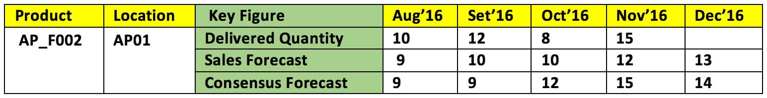 Figure 1: Simple planning layout
All the fields highlighted in yellow can be classed as Attributes, as we can transform the values of any of these. The fields highlighted in green are key figures, where we can define calculations and formulas. Calculations can be done at different planning levels. Finally, the results can be seen in fields in white colour above (basically, values of key figures for the attributes at a planning level).
Let us understand the working principles better with a basic scenario, wherein we need to display the Delivered Quantity from last year in another key figure which demand planners can use for analysis.
So, let’s say we have a key figure for Delivered Qty in our System that we want to show the data from last year in the same view.
![]() Figure 2: Dataset to be used
Figure 2: Dataset to be used
The data displayed in ‘Delivered Qty Last Year’ is same as actuals as already present in key figure ‘Delivered Qty’, but on the past time horizon. So, we transform the time bucket of the key figure ‘Delivered Qty Last year’ (In above case months by 12 months in future). Highlighted in red above.
To achieve this, we follow 4 step process mentioned below;
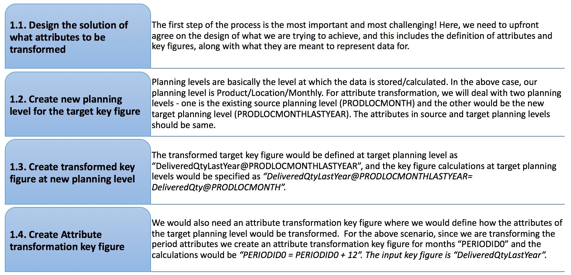 Figure 3: Four step Attribute Transformation Process
Now, when the calculation of the keyfigure “Delivered Qty Last Year” is run, the Period ID of planning level PRODLOCMONTHLASTYEAR is already transformed by + 12 months, hence the above calculations will copy value from Aug/Sep/Oct’16 from key figure “DeliveredQty” and will show the values in Aug/Sep/Oct’17 in “Delivered Qty Last Year”.
 Figure 4: Example where we have transformed last year’s sales quantity and revenue
Attribute Transformations can also answer questions like how will I show aggregated values for all previous months (like what we see in initial bucket in SAP APO SNP planning area).
Power of Attribute Transformations
Enough said about time based Attribute Transformations, let’s talk about what other things we can do with other datasets. As we can transform a time bucket, can I also transform any of other attributes like Product or Location? The answer is of course yes. With Attribute Transformations, we can convert any attribute, be it of either Time, Product, Location or Customer dimension.
Distribution centre closure
Let’s consider a business case where one of our depots is being replaced by another depot. Here, I would need to transfer all my demand from closing (source) depot to new (target) depot. In APO DP, this can be done using realignment, but as at 1608 release, there is no standard functionality within SAP IBP.
So, how can we achieve this scenario within SAP IBP currently? Can we do by using the Lifecycle Management app? Yes, but with limitations. The Lifecycle Management app will only copy and move my statistical forecast, not the final Consensus Demand. Also, I would need to create a lifecycle profile for each source Product-Location combination - which is very tedious.
The answer to this? Attribute Transformation of course! In this case, we can transform the attribute to replace the source location with new target location and hence can move all our forecast to the new depot.
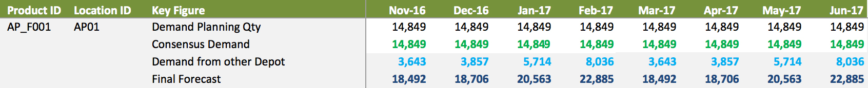 Figure 5: Showing Demand from Another Depot key figure
Dependant Demand Forecast
There are many similar examples for using Attribute Transformations, like complimentary items forecasting. Let’s take an example of a sports equipment company that manufactures tennis racquets and sells them with racquet covers. Now, there will always be a racquet cover with every new tennis racquet sold, but the racquet cover can also be sold as a spare single item (note this is not a DP BoM scenario where we have a parent and a child, but rather it is about generating a complimentary forecast). So, in such a scenario, we can generate a complimentary forecast for the racquet cover which is derived from both the demand of the spare single item sales, but also the requirements generated through new racquet sales. Let’s say spare covers only sell 200 units a year, but the sale new of tennis racquets is 2000 a year - so, in this case the total demand for racquet cover would be 2200, of which 200 units as a standalone unit and 2000 units as dependant demand based on tennis racquet sales.
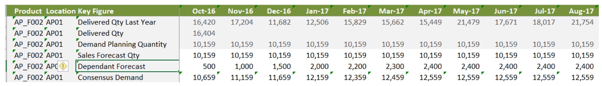 Figure 6: Showing Dependant Demand key figure
Consensus demand is then calculated as the sum of both Dependant and Independent forecasts.
Product Substitution
Another scenario wherein we can use the attribute transformation is Product substitution. Here, we can use an Attribute Transformation on Product ID to substitute one product with a different product ID – akin to Product Interchangeability in APO.
Conclusion
Does this mean the end to custom developments? We have heard this so many times recently from our current and prospective clients that SAP IBP as a cloud based solution means an end to custom developments as we know it. Well the initial answer is obviously yes, due to the fact that the ability for customers to write their own code in IBP is almost zero (we can request SAP to release ‘L-Codes’, but only SAP can write and deliver these). On reflection and second though, we believe it’s not the end of custom developments, but rather a change in mindset from custom developments to configuration. We strongly believe that most of the business scenarios which are currently in APO DP can be modeled within SAP IBP using configuration. Functionalities like Attribute Transformations, Operators and Key Figure based calculations all play their role in achieving the end state of transforming data to the business requirement.
So, just to summarize we all have written numerous custom developments in SAP APO systems to configure such specific scenarios where we needed to change time buckets, or move data between CVCs and/or update navigational attributes. However, with IBP we can manage most of the custom developments by innovative configurations in our planning area.
Although we believe development items such as Realignment and Phase-in/out functionalities are on the road map for future releases of SAP IBP, we have shown above the power of Attribute Transformations in replicating Realignment and Phase-in/out capabilities in our internal 1608 IBP system. Creative and improved ways of thinking - that’s the new SAP IBP way!
I do hope this blog was helpful, please do share your views.
10 Comments
You must be a registered user to add a comment. If you've already registered, sign in. Otherwise, register and sign in.
Labels in this area
-
aATP
1 -
ABAP Programming
1 -
Activate Credit Management Basic Steps
1 -
Adverse media monitoring
1 -
Alerts
1 -
Ausnahmehandling
1 -
bank statements
1 -
Bin Sorting sequence deletion
1 -
Bin Sorting upload
1 -
BP NUMBER RANGE
1 -
Business partner creation failed for organizational unit
1 -
Business Technology Platform
1 -
Central Purchasing
1 -
Charge Calculation
2 -
Cloud Extensibility
1 -
Compliance
1 -
Controlling
1 -
Controlling Area
1 -
Data Enrichment
1 -
DIGITAL MANUFACTURING
1 -
digital transformation
1 -
Dimensional Weight
1 -
Direct Outbound Delivery
1 -
E-Mail
1 -
ETA
1 -
EWM
6 -
EWM - Delivery Processing
2 -
EWM - Goods Movement
3 -
EWM Outbound configuration
1 -
EWM-RF
1 -
EWM-TM-Integration
1 -
Extended Warehouse Management (EWM)
3 -
Extended Warehouse Management(EWM)
7 -
Finance
1 -
Freight Settlement
1 -
Geo-coordinates
1 -
Geo-routing
1 -
Geocoding
1 -
Geographic Information System
1 -
GIS
1 -
Goods Issue
2 -
GTT
2 -
IBP inventory optimization
1 -
inbound delivery printing
1 -
Incoterm
1 -
Innovation
1 -
Inspection lot
1 -
intraday
1 -
Introduction
1 -
Inventory Management
1 -
Logistics Optimization
1 -
Map Integration
1 -
Material Management
1 -
Materials Management
1 -
MFS
1 -
Outbound with LOSC and POSC
1 -
Packaging
1 -
PPF
1 -
PPOCE
1 -
PPOME
1 -
print profile
1 -
Process Controllers
1 -
Production process
1 -
QM
1 -
QM in procurement
1 -
Real-time Geopositioning
1 -
Risk management
1 -
S4 HANA
1 -
S4-FSCM-Custom Credit Check Rule and Custom Credit Check Step
1 -
S4SCSD
1 -
Sales and Distribution
1 -
SAP DMC
1 -
SAP ERP
1 -
SAP Extended Warehouse Management
2 -
SAP Hana Spatial Services
1 -
SAP IBP IO
1 -
SAP MM
1 -
sap production planning
1 -
SAP QM
1 -
SAP REM
1 -
SAP repetiative
1 -
SAP S4HANA
1 -
SAP Transportation Management
2 -
SAP Variant configuration (LO-VC)
1 -
Source inspection
1 -
Storage bin Capacity
1 -
Supply Chain
1 -
Supply Chain Disruption
1 -
Supply Chain for Secondary Distribution
1 -
Technology Updates
1 -
TMS
1 -
Transportation Cockpit
1 -
Transportation Management
2 -
Visibility
2 -
warehouse door
1 -
WOCR
1
Related Content
- What's new in SAP Asset Performance Management 2402 in Supply Chain Management Blogs by SAP
- Transforming Cell Gene Therapy Operations: The Power of Integrated Scheduling and Resource Planning Systems in Supply Chain Management Blogs by SAP
- Supplier Integration between SAP IBP and SAP Business Networks in Supply Chain Management Blogs by SAP
- How to Make Your Clinical Distribution More Efficient in Supply Chain Management Blogs by SAP
- SAP Customer Engagement Initiative Projects for SAP Supply Chain Management - Register until June 16, 2023 in Supply Chain Management Blogs by SAP
Top kudoed authors
| User | Count |
|---|---|
| 2 | |
| 1 | |
| 1 | |
| 1 | |
| 1 | |
| 1 | |
| 1 | |
| 1 | |
| 1 | |
| 1 |