
- SAP Community
- Groups
- Interest Groups
- Application Development
- Blog Posts
- To buffer or not to buffer a database table?
Application Development Blog Posts
Learn and share on deeper, cross technology development topics such as integration and connectivity, automation, cloud extensibility, developing at scale, and security.
Turn on suggestions
Auto-suggest helps you quickly narrow down your search results by suggesting possible matches as you type.
Showing results for
former_member18
Participant
Options
- Subscribe to RSS Feed
- Mark as New
- Mark as Read
- Bookmark
- Subscribe
- Printer Friendly Page
- Report Inappropriate Content
08-27-2015
5:23 PM
It is common knowledge that buffering of database tables improves the system performance, provided the buffering is done judiciously – i.e. only those tables that are read frequently and updated rarely are buffered. But how exactly can we determine if a table is read frequently or updated rarely?
Also, the state of a buffered table in the buffer area is a runtime property which keeps changing with time. How can an ABAP developer, know whether a buffered table actually exists in the buffer, at a given time instant? This is a critical question to be considered while analyzing the performance of queries on buffered tables.
This blog post attempts to answer the above questions.
This blog post is divided into 3 sections and structured as follows:
- Section 1: Prerequisites (Recap of Table Buffering Fundamentals and its Mechanism)
- Section 2: How to use the Table Call Statistics Transaction
- Section 3: Interpreting the results of the Table Call Statistics Transaction to answer the questions posed above.
:!: You might find the blog to be slightly lengthy but the content will NOT be more than what you can chew. Trust me! :grin:
Section 1: Prerequisites (Recap of Table Buffering Fundamentals and its Mechanism)
Buffering is the processing of storing table data (which is always present in the database) temporarily in the RAM of the Application Server. Buffering is specified in the technical settings of a table’s definition in the DDIC.
The benefits of buffering are:
- Faster query execution – A query is atleast 10 times faster when it fetches data from the buffer as compared to a query fetching data from the database. This is because the delays involved in waiting for the database and the network that connects it, are eliminated. The performance of the application which uses this query, is improved.
- Reduced DB Load and Reduced Network Traffic – Since every query need not hit the DB, the load on the DB is reduced and also the network traffic between the Application Layer and the Database Layer is reduced. This improves the performance of the entire system.
The buffering mechanism can be visualized in Figure 1 below:

Figure 1: Buffering Mechanism
The SAP work processes of an application server have access to the SAP table buffer. The buffers are loaded on demand via the database connection. If a SELECT statement is executed on a table selected for buffering, the SAP work process initially looks up the desired data in the SAP table buffer. If the data is not available in the buffer, it is loaded from the database, stored in the table buffer, and then copied to the ABAP program (in the internal session). Subsequent accesses to this table would fetch the data from the buffer and the query need not go to the database to fetch it.
It must be understood that RAM space in the application server is limited. Let’s say – dbtab1 is a buffered table whose data is present in the buffer. When there is a query on another buffered table - dbtab2, its data will have to be loaded into the buffer. This might result in the data of dbtab1 getting displaced from the buffer.
When there is a write access to a buffered table, the change is done in the database and the old table data which is present in the buffer (of the application server from which the change query originated) is just flagged as “Invalid”. At this instant, the buffer and the database hold different data for the same table. A subsequent read access to the table would initiate a reload of the table data from the database to the buffer. Now the buffer holds the same data as the database.
Buffering a table that gets updated very frequently might actually end up increasing the load on the DB and increasing the network traffic between the application layer and the database. This would slow down the system performance and defeat the purpose of buffering.
Key Takeaways from Section 1:
- The contents of a buffered table in the buffer area is completely runtime dependent. At one instant, there might be data, and at another instant, it might not be present.
- Only a table with the following characteristics must be buffered:
(a) Read frequently
(b) Updated rarely
(c) Contains less data
Section 2: How to use the Table Call Statistics Transaction
This is accessed by the Tcode – ST10. The following is the initial screen:
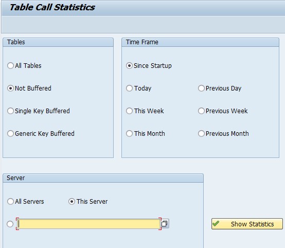
Figure 2: ST10 - Initial Screen
A few points may be noted in Figure 2:
- An access to every table, regardless of whether it is non-buffered/single record buffered/generic area buffered/fully buffered, would be reported by this transaction.
- Analysis of the table accesses may be restricted to a specified time frame (by choosing the radiobuttons - This day/Previous Day/This Month/Previous Month etc). Or the transaction may be run without any restriction on the time period by choosing - “Since Startup”.
- If the SAP system consists of multiple application servers, the accesses (i.e. queries) to the tables originating from any of the servers can be reported by this transaction. On the other hand, the transaction may be restricted to table accesses originating from a specific server (by either choosing the radiobutton – “This Server” or by explicitly specifying the server).
Let’s explore the results returned by the transaction when the radiobutton – “Not Buffered” is chosen.

Figure 3: Results of ST10 when the radio buttons - “Non-Buffered”, “This Server” and “From startup” are chosen
Let me explain the significance of each column –
- Direct Reads – This gives the number of SELECT queries on a particular table in which the entire primary key was specified in the WHERE clause.
- Seq. Reads – This gives the number of SELECT queries on a particular table in which the entire primary key was NOT specified in the WHERE clause. There can more than one record satisfying the WHERE clause.
- Changes – This gives the number of write access (INSERT/UPDATE/MODIFY/DELETE) on a particular table.
- Total – This is the total number of accesses (read + write) to a particular table in the time frame chosen and in the server chosen.
Total = Direct Read + Seq. Reads + Changes.
- Changes/Total % = Also termed as “Change Rate”, this is the % of accesses that are write accesses.
- Rows Affected – This not very relevant for an ABAP developer. Any operation that accesses the database will increase the Rows Affected. SWAPS would also increase this count.
Let’s explore the results when the radio button – “Generic Key Buffered” is chosen:
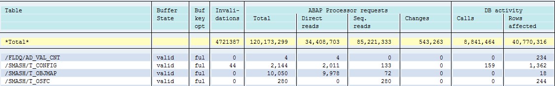
Figure 4: Results of ST10 when the radio buttons - “Generic Key Buffered”, “This Server” and “From startup” are chosen
There are some new columns here, which were not present in Figure 3. They are:
- Buf key opt – This describes the buffering type of the table. Its possible values are:
(a) SNG – Single Record Buffered Table
(b) FUL – Fully Buffered Table
(c) GEN – Generic Area Buffered Table
- Buffer State – This describes the state of the table in the buffer. For all the possible values and their meaning, I would recommend you to just place the cursor on this column and hit F1. The following is a brief description of some of the possible values of Buffer State:
(a) VALID - The table content in the buffer is valid. Read access takes place in the buffer.
(b) ABSENT – The table has not been accessed yet. So the table buffer is not yet loaded with data.
(c) DISPLACED – The table buffer has been displaced
(d) INVALID - The table content is invalid and there are open transactions that modify the table content. Read access takes place in the database.
(e) ERROR - The table content could not be placed in the buffer, because insufficient space.
(f) LOADABLE – The table buffer in the buffer area is invalid, but can be loaded in the next access.
(g) MULTIPLE – Relevant only in the context of Generic Area Buffered Tables. These have different buffer statuses.
- Invalidations: Specifies how often the table was invalidated because of “Changes” (i.e. write accesses).
NOTE: All the table buffers in the current application server can be cleared by entering the Tcode- “/$TAB”.
Note that the user can toggle between one result set and another by using the buttons in the Application Toolbar (as shown in Figure 5):

Figure 5: Application Toolbar of the primary list screen of ST10.
- While the result screen of ST10 may be open in one session, there may be some accesses to tables in other sessions or by other users. Use the “Refresh” button so that the transaction shows the latest data – latest buffer state of tables, latest no. of accesses etc.
- “Reset” button will set all the counts to zero (i.e. no. of reads/changes/DB Calls etc).
- Detailed information about Buffer Administration etc may be viewed by double clicking on any of the entry, or placing the cursor on a row and clicking the “Choose” button on the application toolbar. The secondary list will look like Figure 6.

Figure 6: Secondary List
Section 3: Interpreting the results of the Table Call Statistics Transaction to answer the questions posed above.
How to determine a non-buffered table which is suited to be buffered?
- Begin the ST10 transaction by clicking on the “Non-Buffered” radiobutton.
- Notice the “Change Rate” value for each table. The higher the Change Rate for a table, the less suited it is for buffering.
- The non-buffered tables with the following properties may be considered for buffering:
(a) Low Change Rate (under 0.5%)
(b) High number of reads (Direct Reads + Seq.Reads)
(c) Data volume not too large
If it is to be buffered, what should be its buffering type?
- We are to be guided by the relative number of Direct Reads and Seq. Reads. If most of the reads are Direct Reads, categorize the table as “Single Record Buffered”.
- On the other hand, if most of the reads are Seq. Reads, classify it as either Generic Area Buffered or Fully Buffered. If the data volume is less, the table can be considered for Full Buffering. If the data volume is higher or if certain “groups” of data of this table are accessed frequently, then classify it as “Generic Area Buffered”.
How to determine the efficiency of the buffer setting of already buffered tables?
- Begin the ST10 transaction by clicking on either the “Generic Key Buffered” or “Single Record Buffered” radiobutton (depending upon the table whose buffer setting, you would like to verify).
- Notice the “Change Rate” value for each table. The higher the Change Rate for a table, the less suited it is for buffering. One might consider switching OFF the buffering for such tables.
- A wrong decision with respect to the Buffering Type may also be diagnosed here. For a Single Record Buffered table, if the no. of Seq. Reads is higher relative to the number of Direct Reads, one might consider changing the buffering type from Single Record to Fully Buffered or Generic Area Buffered.
NOTE: Ensure that the time frame for which the transaction is run is significant enough such that all the reports/applications were run in that period and all business scenarios occurred in that period. Only then, can this transaction guide us effectively in deciding which table’s buffer settings are to be altered.
Case Study:
Based on the above guidelines, let’s consider some examples in Figure 7, which shows the Non-Buffered Tables:

Figure 7: List of accesses to non-buffered tables.
I would like to draw your attention to the 3 tables enclosed by a green rectangle. Based on the trends for these three tables, it can be temporarily concluded that:
- The table – ABDBG_LISTENER is NOT a candidate for buffering. This is because, it has a high change rate.
- The table – ABDBG_INFO can be considered for buffering and it may be set as “Single Record Buffered” table since all of its accesses were Direct Reads.
- The table – ADCP can be considered for either Full Buffering or Generic Area Buffering. This is because most of its accesses were Seq. Reads.
The above points are not the final decisions but just guidelines. Other aspects like data volume, size category, access frequency etc are to be considered.
How can an ABAP developer, know whether a buffered table actually exists in the buffer, at a given time instant?
- Clear all the table buffers from the buffer area by running the tcode – “/$TAB”.
- Consider the single record buffer table – TSTC. Its buffer state would say – LOADABLE as shown in Figure 8 below:

Figure 8: Buffer State of TSTC table after clearing the buffers using - /$TAB.
- Now, run the following code snippet in a program:
DATA: GW_TSTC TYPE TSTC.
CONSTANTS: C_SE38 TYPE TSTC-TCODE VALUE 'SE38'.
SELECT SINGLE *
FROM TSTC
INTO GW_TSTC
WHERE TCODE = C_SE38.
- After running the above code snippet, press the “Refresh” button in the Application Toolbar of the ST10 transaction. This would reflect the new buffer state of the TSTC table – VALID.

Figure 9: Buffer State of TSTC table after the above code snippet is run
- Basically, the SELECT SINGLE query first looked for the relevant record in TSTC’s table buffer first. It did not find it (because the table buffer had no data. Its state was LOADABLE earlier). Then, the query fetches the relevant record from the database (this fact can be confirmed from the ST05 – SQL Trace in Figure 10) and loads that data to the buffer.

Figure 10: ST05-SQL Trace when the above code snippet is run for the first time. Data is fetched from database.
- The subsequent reads to TSTC, looking for the same record (i.e. TCODE = ‘SE38’) would fetch the data from the buffer itself (This fact can be confirmed from ST05 – Buffer Trace in Figure 11 This fetch would be several times faster than fetching from the DB.

Figure 11: ST05-Buffer Trace when the above code snippet is run for the second time. Data is fetched from buffer.
Conclusion:
ST10 is a very useful transaction that can guide you in answering the following questions:
- Based on the accesses over a period of time from a particular server, can a non-buffered be buffered?
- Can a table that was wrongly buffered, be identified?
- How can an ABAP developer, know whether a buffered table actually exists in the buffer, at a given time instant?
References:
[1] Gahm, H., “Chapter 3 – Performance Analysis Tools,” ABAP Performance Tuning, 1st ed., Galileo Press, Boston, 2010, pp. 51-54.
- SAP Managed Tags:
- ABAP Testing and Analysis
7 Comments
You must be a registered user to add a comment. If you've already registered, sign in. Otherwise, register and sign in.
Labels in this area
-
A Dynamic Memory Allocation Tool
1 -
ABAP
8 -
abap cds
1 -
ABAP CDS Views
14 -
ABAP class
1 -
ABAP Cloud
1 -
ABAP Development
4 -
ABAP in Eclipse
1 -
ABAP Keyword Documentation
2 -
ABAP OOABAP
2 -
ABAP Programming
1 -
abap technical
1 -
ABAP test cockpit
7 -
ABAP test cokpit
1 -
ADT
1 -
Advanced Event Mesh
1 -
AEM
1 -
AI
1 -
API and Integration
1 -
APIs
8 -
APIs ABAP
1 -
App Dev and Integration
1 -
Application Development
2 -
application job
1 -
archivelinks
1 -
Automation
4 -
BTP
1 -
CAP
1 -
CAPM
1 -
Career Development
3 -
CL_GUI_FRONTEND_SERVICES
1 -
CL_SALV_TABLE
1 -
Cloud Extensibility
8 -
Cloud Native
7 -
Cloud Platform Integration
1 -
CloudEvents
2 -
CMIS
1 -
Connection
1 -
container
1 -
Debugging
2 -
Developer extensibility
1 -
Developing at Scale
4 -
DMS
1 -
dynamic logpoints
1 -
Eclipse ADT ABAP Development Tools
1 -
EDA
1 -
Event Mesh
1 -
Expert
1 -
Field Symbols in ABAP
1 -
Fiori
1 -
Fiori App Extension
1 -
Forms & Templates
1 -
IBM watsonx
1 -
Integration & Connectivity
10 -
JavaScripts used by Adobe Forms
1 -
joule
1 -
NodeJS
1 -
ODATA
3 -
OOABAP
3 -
Outbound queue
1 -
Product Updates
1 -
Programming Models
13 -
Restful webservices Using POST MAN
1 -
RFC
1 -
RFFOEDI1
1 -
SAP BAS
1 -
SAP BTP
1 -
SAP Build
1 -
SAP Build apps
1 -
SAP Build CodeJam
1 -
SAP CodeTalk
1 -
SAP Odata
1 -
SAP UI5
1 -
SAP UI5 Custom Library
1 -
SAPEnhancements
1 -
SapMachine
1 -
security
3 -
text editor
1 -
Tools
16 -
User Experience
5
Top kudoed authors
| User | Count |
|---|---|
| 5 | |
| 5 | |
| 3 | |
| 3 | |
| 2 | |
| 2 | |
| 2 | |
| 2 | |
| 1 | |
| 1 |