
- SAP Community
- Products and Technology
- Technology
- Technology Blogs by Members
- Backend Performance Tips
Technology Blogs by Members
Explore a vibrant mix of technical expertise, industry insights, and tech buzz in member blogs covering SAP products, technology, and events. Get in the mix!
Turn on suggestions
Auto-suggest helps you quickly narrow down your search results by suggesting possible matches as you type.
Showing results for
celo_berger
Active Participant
Options
- Subscribe to RSS Feed
- Mark as New
- Mark as Read
- Bookmark
- Subscribe
- Printer Friendly Page
- Report Inappropriate Content
04-08-2015
9:29 PM
Overview
Performance tuning is always a consideration when building data warehouses. The expected tendency is for a DW DB to grow, as data is being added on a daily basis. And as the volume increases, performance will decrease as reports are now querying millions of records across multiple years.
The purpose of this document is to focus on a few backend performance best practices and tricks that I’ve learned across the years, that will save time during ETL, and as a result, will be an overall more efficient DW to serve the clients reporting interests.
Many of these topics have been covered here on SCN, some not so much. This is by no means a comprehensive list and is a consolidation of what I’ve found most useful in my projects.
For full disclosure, I’m not an ABAPer and my ABAP knowledge is limited. So the basis for my recommendations are purely based on performance comparisons before and after the ABAP changes referenced in this post. I’m sure that you can find many blogs and forums around each of topics I’ll be mentioning.
Logical Partitioning
As your data warehouse matures, and your data is now many years old, you might find yourself stuck with a cube that contains multiple years of data. If best practices were followed, you should have a multiprovider on top of your cube for the reporting layer:

There are a few disadvantages to having a single cube storing multiple years of data:
- Increased loading time
- Increased reload time if changes are required, such as a new field being added (all history needs to be reloaded)
- Decreased query performance, as the select from BEx will sift through all the records in the cube
Logically Partitioned cubes are exactly what the name suggests: partitioning (or splitting) the data in the cube according to a logical criteria. The example I will give below is an easy to understand one, but it can really be done by any field that doesn’t have too many dimensions to it.
What I’ve done in the past, was to logically partition cubes based on the Fiscal Year/Calendar Year. In this scenario, you’d have multiple infocubes logically partitioned by year, 2010, 2011…..2017, 2018 etc. All the cubes would be linked together through a single multiprovider:

This option does require a little setup, such as creating transformations and DTPs for each cube, and ensuring the correct data is being loaded to each cube, either through a simple start routine that deletes the SOURCE_PACKAGE where CALYEAR NOT “YYYY”, or by having filters in the DTPs that only load the appropriate year into each cube.
But once the setup is done, if data reloads are required for specific years, you only need to reload that particular cube, without disrupting reporting on all the other data.
When running a report with data for a single year, the multiprovider will be smart enough to direct the select statement to the appropriate cube, thus eliminating data from the other years that will not be queried, and improving report run times.
This practice is the most recommended, so much so that SAP provided a standard functionality to accomplish that, which is topic of the next segment:
Semantic Partitioned Objects
SPOs are the exact same concept as logical partitioning. SAP provided functionality to enable partitioning in BW in a more streamlined and automated way.
The link below provides a great how-to guide on using SPOs by Rakesh Dilip Kalyankar:
http://www.sdn.sap.com/irj/scn/go/portal/prtroot/docs/library/uuid/50e09876-d902-2f10-1db6-ce161ab7f...
Batch Jobs for DTP Executions
As part of ETL, BW developers will schedule DTPs to be executed. Depending on the size and complexity of the process chains, as well as the number of available background jobs at any given time, we can take advantage of having multiple parallel background jobs to be run per DTP.
There isn’t a straightforward number of parallel jobs that should be set, since each BW system is unique, in terms of:
- Amount of infoproviders that need to be loaded
- Availability and number of background jobs
- Timing in which loads need to be completed
- Number of DTPs scheduled to run in parallel via process chains
Although one main rule is that the number of jobs has to be multiples of 3 for transactional data, and we can only have 1 job for master data.
To change the background job settings, in the menu, click on Goto -> Settings for Batch Manager …

Change the Number of Processes number to increase or decrease the number of background jobs

Here are a few tips on how to determine the number of background jobs to set for a particular DTP:
1. Assess the volume and criticality of the load:
a. Higher volume and critical loads (loads that need to be completed before 8AM or when the business needs the data) should have more parallel background jobs. A ballpark number I’ve used is between 9-12 background jobs.
b. If, for example, you have a DTP load that on a daily basis takes 4 hours and is holding the entire process chain down, it might be a candidate for increasing background jobs.
2. Determine the amount of available background jobs by going to SM51 and double clicking on the available servers, and viewing the total background jobs

With that number, you have an estimate of how many background jobs you can parallelize.
*Important: if you have 20 total background jobs, you should NOT try to max out and consume those 20 jobs. Try and stay 2-3 jobs below that threshold so you don’t get into job queuing issues which could lead to loss of performance
3. Assess the process chains in your system to identify where loads can be parallelized and where it makes sense to increase the number of background jobs in the DTPs
DTP Data Package Size
Many times overlooked, the Package Size can provide moderate to significant performance improvements if tweaked correctly.
Typically a larger package size is preferable, since the overhead to initialize each data packet is reduced, since more records are being bundled into a single package.
For example, if we’re loading 50k records from a PSA to a DSO:
1. Package size of 1000:
a. This results in 50x overhead since the DTP is going to load 50 packages of 1000 to load 50k;
2. Package size of 50000:
a. Only one overhead processing since we’re grouping all the records into a single 50k package.
Option 2 will provide better performance

However, there are some considerations when modifying the package size:
1. If there’s custom logic in the transformation to do large volume lookups from other DSOs or Master Data objects, it might be necessary to reduce the package size, since there’s a limit to how much memory can be used for internal tables. If the level of complexity or data volume in the custom code is so great, then that might be the only option to ensuring the loads complete successfully. And you will only find out through trial and error;
2. If there’s no custom code or logic in the transformation, it is possible to expand the package size by 5-10x the default setting of 50k. Again, trial and error will help determine the sweet spot.
Secondary Indices on DSOs
Another common issue observed was around poor performance in transformations when doing non key selects from DSOs. Fortunately SAP provides a very simple fix for that, which is the ability to create Secondary Indices on DSOs.
It’s a very simple process, which will improve the performance in those selects tremendously.
In the DSO modelling screen (double clicking on the DSO)

At the bottom, under Indexes, right click and select Create New Indexes

Leave the Unique checkbox unchecked. If checked, the secondary index which is being created would have to have unique values in the DSO, which might not be the case, if for example the index is being created on the GL Account field. There could be multiple records in the DSO with the same GL Account.


Once created, simply drag a field from the Data Fields into the new index, and activate the DSO

Master Data Lookup in Transformation
SAP introduced a nice functionality that automatically allows us, without any code, to select master data attributes in the field routine of transformations:
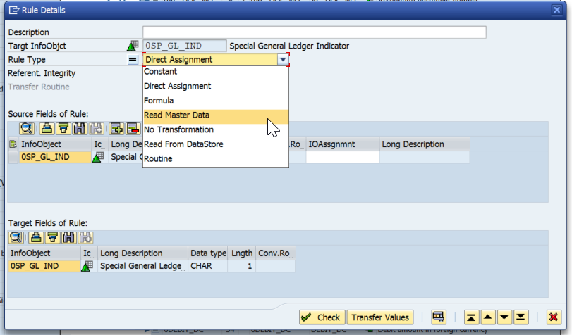
This simplifies the build process significantly, as no code is required.
However, we’ve noticed that this actually decreases the loading performance compared to doing a select statement in the start routine, and then reading the internal table in the field routines, as the example below:
START ROUTINE
SELECT FIELD1 FIELD2
FROM /BI0/PFIELD1
INTO TABLE itab1
FOR ALL ENTRIES IN SOURCE_PACKAGE
WHERE FIELD1 = SOURCE_PACKAGE-FIELD1 AND
objvers = 'A'.
FIELD ROUTINE
IF RESULT_FIELDS IS NOT INITIAL.
READ TABLE ITAB1 WITH TABLE KEY
FIELD1 = RESULT_FIELDS-FIELD1 ASSIGNING <f_s_itab1>.
IF <f_s_itab1> IS ASSIGNED.
RESULT = <f_s_itab1>-FIELD2.
UNASSIGN <f_s_itab1>.
ENDIF.
ENDIF.
The reason for that is actually quite simple. If for example, we’re loading 50k records per data package, the single select statement in the start routine will do one select for 50k records and store that in our internal table.
If we use the field routine standard logic, as it is a FIELD routine, it will end up doing 50k selects, which is significantly more costly.
One consideration to keep in mind is for time dependent master data. Given the complexities around figuring out the correct time period to select, I have used the standard SAP functionality of Reading the Master Data in the field routines of the transformations to select time dependent attributes.
Hashed Tables
Hashed tables are nothing but tables that have a defined key, as opposed to a standard table where you need to perform a SORT command in order to do an efficient READ with BINARY-SEARCH.
So when declaring the DATA type, there would be an explicit command:
TYPES: BEGIN OF t_itab1,
field1 TYPE /BI0/OIFIELD1,
field2 TYPE /BI0/OIFIELD2,
END OF t_itab1.
DATA: itab1 TYPE HASHED TABLE OF t_itab1 WITH UNIQUE KEY field1.
FIELD-SYMBOLS: <f_s_itab1> type t_itab1.
For this particular internal table itab1, we know that field1 is unique and therefore we can declare it that way.
When the data is selected, the system will index it according to the specified key. SORTs and BINARY-SEARCH are not required in this case.
Below is an example of a read statement on the hashed table. One thing to keep in mind is to use WITH TABLE KEY for reading hashed tables, as opposed to WITH KEY for standard tables
READ TABLE itab1 WITH TABLE KEY
field1 = RESULT_FIELDS-field1 ASSIGNING <f_s_itab1>.
Field Symbols Instead of Work Areas
A field symbol acts as a pointer to a record in an internal table, whereas a work area actually holds the value from an internal table.
So if we do a loop on an internal table with 100 records, the field symbol will store the position of each record through each pass of the loop, and allow us to modify that internal table, whereas the work area will actually store the record that was looped.
What we’ve noticed is that field symbols provide better performance when having to loop or read through internal tables.
To declare a field symbol, you first need to have a type or structure declared or available:
TYPES: BEGIN OF t_itab1,
field1 TYPE /BI0/OIFIELD1,
field2 TYPE /BI0/OIFIELD2,
END OF t_itab1.
FIELD-SYMBOLS: <f_s_itab1> type t_itab1.
When performing a read you will use the ASSIGNING command:
READ TABLE itab1 WITH TABLE KEY
field1 = RESULT_FIELDS-field1 ASSIGNING <f_s_itab1>.
For validating if the field symbol is assigned:
IF <f_s_itab1> IS ASSIGNED.
Write your logic
Don’t forget to unassign the field symbol after your logic is complete:
UNASSIGN <f_s_itab1>.
And close your IF statement:
ENDIF.
Looping is similar to a read, as you also have to use the ASSIGNING command:
LOOP AT SOURCE_PACKAGE ASSIGNING <source_fields>.
The main difference is that you do NOT need to unassign the field symbol. At each iteration of the loop, it will unassign and reassign to the next record in the internal table.
However, if you do wish to reutilize the field symbol after your ENDLOOP, you should immediately unassign it to prevent incorrect records being pointed to:
LOOP AT SOURCE_PACKAGE ASSIGNING <source_fields>.
Write your logic
ENDLOOP.
UNASSIGN <source_fields>.
Parallel Cursor
Inevitably when writing ABAP code, we will stumble across a scenario where we need to write a loop within a loop. That is a big no-no in terms of ABAP programming best practices. There’s a nifty little trick that’s called a parallel cursor.
Here’s how it works:
1. If you’re not using hashed tables, make sure to sort itab1 and itab2;
2. Start the first loop into itab1 and assign field symbol <fs1>;
3. Within your loop on itab1, we first do a READ into itab2, assigning field symbol <fs2>, to determine the exact location of the record that is required;
4. If a record is found and <fs2> is assigned, we then save the position of the record (sy-tabix) to our variable lv_index;
5. We then unassign <fs2> so we can start the loop with parallel cursor
6. We start the loop into itab2 from that start position lv_index;
7. After assigning <fs2> we do a check to validate if the field1 we’re selecting from the 2nd loop matches the record in <fs1>.
a. If it does, we carry on with our logic;
b. If it doesn’t, we exit, and now we will move on to the next record in itab1
Below is an example of the parallel cursor:
LOOP AT itab1 ASSIGNING <fs1>.
READ TABLE itab2 WITH KEY field1 = <fs1>-field1
ASSIGNING <fs2> BINARY SEARCH.
IF <fs2> IS ASSIGNED.
lv_index = sy-tabix.
UNASSIGN <fs2>.
LOOP AT itab2 ASSIGNING <fs2> FROM lv_index.
IF <fs1>-field1 <> <fs2>-field1
EXIT.
ENDIF.
write your code
ENDLOOP.
ENDLOOP.
And with comments:
LOOP AT itab1 ASSIGNING <fs1>. Our first loop
READ TABLE itab2 WITH KEY field1 = <fs1> ASSIGNING <fs2> BINARY SEARCH. Reading our 2nd internal table we wish to loop into to determine the start position of the second loop
IF <fs2> IS ASSIGNED. If a value is found, it will be assigned and pass this check
lv_index = sy-tabix. Store the position of the found record in itab2
UNASSIGN <fs2>. Clear the field symbol
LOOP AT itab2 ASSIGNING <fs2> FROM lv_index. Start the loop at the position we found above on itab2
IF <fs1>-field1 <> <fs2>-field1 if we’ve now looped through itab2 and it no longer matches the record in <fs1>, it’s time to move to the next record in the loop for itab1, so we exit the 2nd loop on itab2
EXIT. Exits the loop on itab2
ENDIF.
Write your logic for when <fs1>-field1 = <fs2>-field1
ENDLOOP. Endloop for itab2
ENDLOOP. Endloop for itab1
Summary
Hopefully these tips can help you build a more efficient and better performing backend SAP BW data warehouse. Your feedback and suggestions are always welcome, and if you have better or different ways of doing the same thing, I'd definitely be interested in learning them.
Best of luck on your developments!
- SAP Managed Tags:
- BW (SAP Business Warehouse)
7 Comments
You must be a registered user to add a comment. If you've already registered, sign in. Otherwise, register and sign in.
Labels in this area
-
"automatische backups"
1 -
"regelmäßige sicherung"
1 -
"TypeScript" "Development" "FeedBack"
1 -
505 Technology Updates 53
1 -
ABAP
14 -
ABAP API
1 -
ABAP CDS Views
2 -
ABAP CDS Views - BW Extraction
1 -
ABAP CDS Views - CDC (Change Data Capture)
1 -
ABAP class
2 -
ABAP Cloud
2 -
ABAP Development
5 -
ABAP in Eclipse
1 -
ABAP Platform Trial
1 -
ABAP Programming
2 -
abap technical
1 -
absl
2 -
access data from SAP Datasphere directly from Snowflake
1 -
Access data from SAP datasphere to Qliksense
1 -
Accrual
1 -
action
1 -
adapter modules
1 -
Addon
1 -
Adobe Document Services
1 -
ADS
1 -
ADS Config
1 -
ADS with ABAP
1 -
ADS with Java
1 -
ADT
2 -
Advance Shipping and Receiving
1 -
Advanced Event Mesh
3 -
AEM
1 -
AI
7 -
AI Launchpad
1 -
AI Projects
1 -
AIML
9 -
Alert in Sap analytical cloud
1 -
Amazon S3
1 -
Analytical Dataset
1 -
Analytical Model
1 -
Analytics
1 -
Analyze Workload Data
1 -
annotations
1 -
API
1 -
API and Integration
3 -
API Call
2 -
Application Architecture
1 -
Application Development
5 -
Application Development for SAP HANA Cloud
3 -
Applications and Business Processes (AP)
1 -
Artificial Intelligence
1 -
Artificial Intelligence (AI)
5 -
Artificial Intelligence (AI) 1 Business Trends 363 Business Trends 8 Digital Transformation with Cloud ERP (DT) 1 Event Information 462 Event Information 15 Expert Insights 114 Expert Insights 76 Life at SAP 418 Life at SAP 1 Product Updates 4
1 -
Artificial Intelligence (AI) blockchain Data & Analytics
1 -
Artificial Intelligence (AI) blockchain Data & Analytics Intelligent Enterprise
1 -
Artificial Intelligence (AI) blockchain Data & Analytics Intelligent Enterprise Oil Gas IoT Exploration Production
1 -
Artificial Intelligence (AI) blockchain Data & Analytics Intelligent Enterprise sustainability responsibility esg social compliance cybersecurity risk
1 -
ASE
1 -
ASR
2 -
ASUG
1 -
Attachments
1 -
Authorisations
1 -
Automating Processes
1 -
Automation
2 -
aws
2 -
Azure
1 -
Azure AI Studio
1 -
B2B Integration
1 -
Backorder Processing
1 -
Backup
1 -
Backup and Recovery
1 -
Backup schedule
1 -
BADI_MATERIAL_CHECK error message
1 -
Bank
1 -
BAS
1 -
basis
2 -
Basis Monitoring & Tcodes with Key notes
2 -
Batch Management
1 -
BDC
1 -
Best Practice
1 -
bitcoin
1 -
Blockchain
3 -
bodl
1 -
BOP in aATP
1 -
BOP Segments
1 -
BOP Strategies
1 -
BOP Variant
1 -
BPC
1 -
BPC LIVE
1 -
BTP
12 -
BTP Destination
2 -
Business AI
1 -
Business and IT Integration
1 -
Business application stu
1 -
Business Application Studio
1 -
Business Architecture
1 -
Business Communication Services
1 -
Business Continuity
1 -
Business Data Fabric
3 -
Business Partner
12 -
Business Partner Master Data
10 -
Business Technology Platform
2 -
Business Trends
4 -
CA
1 -
calculation view
1 -
CAP
3 -
Capgemini
1 -
CAPM
1 -
Catalyst for Efficiency: Revolutionizing SAP Integration Suite with Artificial Intelligence (AI) and
1 -
CCMS
2 -
CDQ
12 -
CDS
2 -
Cental Finance
1 -
Certificates
1 -
CFL
1 -
Change Management
1 -
chatbot
1 -
chatgpt
3 -
CL_SALV_TABLE
2 -
Class Runner
1 -
Classrunner
1 -
Cloud ALM Monitoring
1 -
Cloud ALM Operations
1 -
cloud connector
1 -
Cloud Extensibility
1 -
Cloud Foundry
4 -
Cloud Integration
6 -
Cloud Platform Integration
2 -
cloudalm
1 -
communication
1 -
Compensation Information Management
1 -
Compensation Management
1 -
Compliance
1 -
Compound Employee API
1 -
Configuration
1 -
Connectors
1 -
Consolidation Extension for SAP Analytics Cloud
2 -
Control Indicators.
1 -
Controller-Service-Repository pattern
1 -
Conversion
1 -
Cosine similarity
1 -
cryptocurrency
1 -
CSI
1 -
ctms
1 -
Custom chatbot
3 -
Custom Destination Service
1 -
custom fields
1 -
Customer Experience
1 -
Customer Journey
1 -
Customizing
1 -
cyber security
3 -
cybersecurity
1 -
Data
1 -
Data & Analytics
1 -
Data Aging
1 -
Data Analytics
2 -
Data and Analytics (DA)
1 -
Data Archiving
1 -
Data Back-up
1 -
Data Flow
1 -
Data Governance
5 -
Data Integration
2 -
Data Quality
12 -
Data Quality Management
12 -
Data Synchronization
1 -
data transfer
1 -
Data Unleashed
1 -
Data Value
8 -
database tables
1 -
Datasphere
3 -
datenbanksicherung
1 -
dba cockpit
1 -
dbacockpit
1 -
Debugging
2 -
Delimiting Pay Components
1 -
Delta Integrations
1 -
Destination
3 -
Destination Service
1 -
Developer extensibility
1 -
Developing with SAP Integration Suite
1 -
Devops
1 -
digital transformation
1 -
Documentation
1 -
Dot Product
1 -
DQM
1 -
dump database
1 -
dump transaction
1 -
e-Invoice
1 -
E4H Conversion
1 -
Eclipse ADT ABAP Development Tools
2 -
edoc
1 -
edocument
1 -
ELA
1 -
Embedded Consolidation
1 -
Embedding
1 -
Embeddings
1 -
Employee Central
1 -
Employee Central Payroll
1 -
Employee Central Time Off
1 -
Employee Information
1 -
Employee Rehires
1 -
Enable Now
1 -
Enable now manager
1 -
endpoint
1 -
Enhancement Request
1 -
Enterprise Architecture
1 -
ETL Business Analytics with SAP Signavio
1 -
Euclidean distance
1 -
Event Dates
1 -
Event Driven Architecture
1 -
Event Mesh
2 -
Event Reason
1 -
EventBasedIntegration
1 -
EWM
1 -
EWM Outbound configuration
1 -
EWM-TM-Integration
1 -
Existing Event Changes
1 -
Expand
1 -
Expert
2 -
Expert Insights
2 -
Exploits
1 -
Fiori
14 -
Fiori Elements
2 -
Fiori SAPUI5
12 -
Flask
1 -
Full Stack
8 -
Funds Management
1 -
General
1 -
General Splitter
1 -
Generative AI
1 -
Getting Started
1 -
GitHub
8 -
Grants Management
1 -
GraphQL
1 -
groovy
1 -
GTP
1 -
HANA
6 -
HANA Cloud
2 -
Hana Cloud Database Integration
2 -
HANA DB
2 -
HANA XS Advanced
1 -
Historical Events
1 -
home labs
1 -
HowTo
1 -
HR Data Management
1 -
html5
8 -
HTML5 Application
1 -
Identity cards validation
1 -
idm
1 -
Implementation
1 -
input parameter
1 -
instant payments
1 -
Integration
3 -
Integration Advisor
1 -
Integration Architecture
1 -
Integration Center
1 -
Integration Suite
1 -
intelligent enterprise
1 -
iot
1 -
Java
1 -
job
1 -
Job Information Changes
1 -
Job-Related Events
1 -
Job_Event_Information
1 -
joule
4 -
Journal Entries
1 -
Just Ask
1 -
Kerberos for ABAP
8 -
Kerberos for JAVA
8 -
KNN
1 -
Launch Wizard
1 -
Learning Content
2 -
Life at SAP
5 -
lightning
1 -
Linear Regression SAP HANA Cloud
1 -
Loading Indicator
1 -
local tax regulations
1 -
LP
1 -
Machine Learning
2 -
Marketing
1 -
Master Data
3 -
Master Data Management
14 -
Maxdb
2 -
MDG
1 -
MDGM
1 -
MDM
1 -
Message box.
1 -
Messages on RF Device
1 -
Microservices Architecture
1 -
Microsoft Universal Print
1 -
Middleware Solutions
1 -
Migration
5 -
ML Model Development
1 -
Modeling in SAP HANA Cloud
8 -
Monitoring
3 -
MTA
1 -
Multi-Record Scenarios
1 -
Multiple Event Triggers
1 -
Myself Transformation
1 -
Neo
1 -
New Event Creation
1 -
New Feature
1 -
Newcomer
1 -
NodeJS
2 -
ODATA
2 -
OData APIs
1 -
odatav2
1 -
ODATAV4
1 -
ODBC
1 -
ODBC Connection
1 -
Onpremise
1 -
open source
2 -
OpenAI API
1 -
Oracle
1 -
PaPM
1 -
PaPM Dynamic Data Copy through Writer function
1 -
PaPM Remote Call
1 -
PAS-C01
1 -
Pay Component Management
1 -
PGP
1 -
Pickle
1 -
PLANNING ARCHITECTURE
1 -
Popup in Sap analytical cloud
1 -
PostgrSQL
1 -
POSTMAN
1 -
Process Automation
2 -
Product Updates
4 -
PSM
1 -
Public Cloud
1 -
Python
4 -
Qlik
1 -
Qualtrics
1 -
RAP
3 -
RAP BO
2 -
Record Deletion
1 -
Recovery
1 -
recurring payments
1 -
redeply
1 -
Release
1 -
Remote Consumption Model
1 -
Replication Flows
1 -
research
1 -
Resilience
1 -
REST
1 -
REST API
2 -
Retagging Required
1 -
Risk
1 -
Rolling Kernel Switch
1 -
route
1 -
rules
1 -
S4 HANA
1 -
S4 HANA Cloud
1 -
S4 HANA On-Premise
1 -
S4HANA
3 -
S4HANA_OP_2023
2 -
SAC
10 -
SAC PLANNING
9 -
SAP
4 -
SAP ABAP
1 -
SAP Advanced Event Mesh
1 -
SAP AI Core
8 -
SAP AI Launchpad
8 -
SAP Analytic Cloud Compass
1 -
Sap Analytical Cloud
1 -
SAP Analytics Cloud
4 -
SAP Analytics Cloud for Consolidation
3 -
SAP Analytics Cloud Story
1 -
SAP analytics clouds
1 -
SAP BAS
1 -
SAP Basis
6 -
SAP BODS
1 -
SAP BODS certification.
1 -
SAP BTP
21 -
SAP BTP Build Work Zone
2 -
SAP BTP Cloud Foundry
6 -
SAP BTP Costing
1 -
SAP BTP CTMS
1 -
SAP BTP Innovation
1 -
SAP BTP Migration Tool
1 -
SAP BTP SDK IOS
1 -
SAP Build
11 -
SAP Build App
1 -
SAP Build apps
1 -
SAP Build CodeJam
1 -
SAP Build Process Automation
3 -
SAP Build work zone
10 -
SAP Business Objects Platform
1 -
SAP Business Technology
2 -
SAP Business Technology Platform (XP)
1 -
sap bw
1 -
SAP CAP
2 -
SAP CDC
1 -
SAP CDP
1 -
SAP CDS VIEW
1 -
SAP Certification
1 -
SAP Cloud ALM
4 -
SAP Cloud Application Programming Model
1 -
SAP Cloud Integration for Data Services
1 -
SAP cloud platform
8 -
SAP Companion
1 -
SAP CPI
3 -
SAP CPI (Cloud Platform Integration)
2 -
SAP CPI Discover tab
1 -
sap credential store
1 -
SAP Customer Data Cloud
1 -
SAP Customer Data Platform
1 -
SAP Data Intelligence
1 -
SAP Data Migration in Retail Industry
1 -
SAP Data Services
1 -
SAP DATABASE
1 -
SAP Dataspher to Non SAP BI tools
1 -
SAP Datasphere
9 -
SAP DRC
1 -
SAP EWM
1 -
SAP Fiori
3 -
SAP Fiori App Embedding
1 -
Sap Fiori Extension Project Using BAS
1 -
SAP GRC
1 -
SAP HANA
1 -
SAP HCM (Human Capital Management)
1 -
SAP HR Solutions
1 -
SAP IDM
1 -
SAP Integration Suite
9 -
SAP Integrations
4 -
SAP iRPA
2 -
SAP LAGGING AND SLOW
1 -
SAP Learning Class
1 -
SAP Learning Hub
1 -
SAP Master Data
1 -
SAP Odata
2 -
SAP on Azure
1 -
SAP PartnerEdge
1 -
sap partners
1 -
SAP Password Reset
1 -
SAP PO Migration
1 -
SAP Prepackaged Content
1 -
SAP Process Automation
2 -
SAP Process Integration
2 -
SAP Process Orchestration
1 -
SAP S4HANA
2 -
SAP S4HANA Cloud
1 -
SAP S4HANA Cloud for Finance
1 -
SAP S4HANA Cloud private edition
1 -
SAP Sandbox
1 -
SAP STMS
1 -
SAP successfactors
3 -
SAP SuccessFactors HXM Core
1 -
SAP Time
1 -
SAP TM
2 -
SAP Trading Partner Management
1 -
SAP UI5
1 -
SAP Upgrade
1 -
SAP Utilities
1 -
SAP-GUI
8 -
SAP_COM_0276
1 -
SAPBTP
1 -
SAPCPI
1 -
SAPEWM
1 -
sapmentors
1 -
saponaws
2 -
SAPS4HANA
1 -
SAPUI5
5 -
schedule
1 -
Script Operator
1 -
Secure Login Client Setup
8 -
security
9 -
Selenium Testing
1 -
Self Transformation
1 -
Self-Transformation
1 -
SEN
1 -
SEN Manager
1 -
service
1 -
SET_CELL_TYPE
1 -
SET_CELL_TYPE_COLUMN
1 -
SFTP scenario
2 -
Simplex
1 -
Single Sign On
8 -
Singlesource
1 -
SKLearn
1 -
Slow loading
1 -
soap
1 -
Software Development
1 -
SOLMAN
1 -
solman 7.2
2 -
Solution Manager
3 -
sp_dumpdb
1 -
sp_dumptrans
1 -
SQL
1 -
sql script
1 -
SSL
8 -
SSO
8 -
Substring function
1 -
SuccessFactors
1 -
SuccessFactors Platform
1 -
SuccessFactors Time Tracking
1 -
Sybase
1 -
system copy method
1 -
System owner
1 -
Table splitting
1 -
Tax Integration
1 -
Technical article
1 -
Technical articles
1 -
Technology Updates
14 -
Technology Updates
1 -
Technology_Updates
1 -
terraform
1 -
Threats
2 -
Time Collectors
1 -
Time Off
2 -
Time Sheet
1 -
Time Sheet SAP SuccessFactors Time Tracking
1 -
Tips and tricks
2 -
toggle button
1 -
Tools
1 -
Trainings & Certifications
1 -
Transformation Flow
1 -
Transport in SAP BODS
1 -
Transport Management
1 -
TypeScript
2 -
ui designer
1 -
unbind
1 -
Unified Customer Profile
1 -
UPB
1 -
Use of Parameters for Data Copy in PaPM
1 -
User Unlock
1 -
VA02
1 -
Validations
1 -
Vector Database
2 -
Vector Engine
1 -
Visual Studio Code
1 -
VSCode
1 -
Vulnerabilities
1 -
Web SDK
1 -
work zone
1 -
workload
1 -
xsa
1 -
XSA Refresh
1
- « Previous
- Next »
Related Content
- ABAP Cloud Developer Trial 2022 Available Now in Technology Blogs by SAP
- Recap - SAP ALM at SAP Insider Las Vegas 2024 in Technology Blogs by SAP
- Unveiling Customer Needs: SAP Signavio Community supporting our customer`s adoption in Technology Blogs by SAP
- SAP Datasphere - Space, Data Integration, and Data Modeling Best Practices in Technology Blogs by SAP
- SAP CAP and SAPUI5 Hierarchy for Tree Table, how to implement hierarchy-node-descendant-count? in Technology Q&A
Top kudoed authors
| User | Count |
|---|---|
| 8 | |
| 5 | |
| 5 | |
| 4 | |
| 4 | |
| 4 | |
| 4 | |
| 4 | |
| 3 | |
| 3 |