
- SAP Community
- Products and Technology
- Technology
- Technology Blogs by SAP
- Play the game of life with SAP HANA
Technology Blogs by SAP
Learn how to extend and personalize SAP applications. Follow the SAP technology blog for insights into SAP BTP, ABAP, SAP Analytics Cloud, SAP HANA, and more.
Turn on suggestions
Auto-suggest helps you quickly narrow down your search results by suggesting possible matches as you type.
Showing results for
Former Member
Options
- Subscribe to RSS Feed
- Mark as New
- Mark as Read
- Bookmark
- Subscribe
- Printer Friendly Page
- Report Inappropriate Content
10-08-2014
11:19 AM
Hi everyone, welcome to the game of life! In this blog, let's play the game of life with SAP HANA. Have fun! :cool:
What is the game of life?
So first of all, what is the game of life? You can find rules of the game of life from Wikipedia as follows.
"The universe of the Game of Life is an infinite two-dimensional orthogonal grid of square cells, each of which is in one of two possible states, alive or dead. Every cell interacts with its eight neighbours, which are the cells that are horizontally, vertically, or diagonally adjacent. At each step in time, the following transitions occur:
1. Any live cell with fewer than two live neighbours dies, as if caused by under-population.
2. Any live cell with two or three live neighbours lives on to the next generation.
3. Any live cell with more than three live neighbours dies, as if by overcrowding.
4. Any dead cell with exactly three live neighbours becomes a live cell, as if by reproduction.
The initial pattern constitutes the seed of the system. The first generation is created by applying the above rules simultaneously to every cell in the seed—births and deaths occur simultaneously, and the discrete moment at which this happens is sometimes called a tick (in other words, each generation is a pure function of the preceding one). The rules continue to be applied repeatedly to create further generations."
Motivation
I still remember when I studied at TU Berlin, I had a course named parallel programming. There was an assignment about the game of life in which we need to implement it with MPI. That's the first time when I heard of the game of life. Since parallelism is one of the powerful weapons owned by SAP HANA, an idea came to my mind, why not play the game of life with SAP HANA? Let's give it a shot.
Problems
Consider the following simple 3x3 initial pattern with live cells shown in black and dead cells shown in white.

According the above rules, the first generation will look like as follows. You can do an exercise yourselves.

Now let's start to play the game of life with SAP HANA. The first thing we need to do is modeling the problem in SAP HANA. For the two-dimensional grid, we can create two axes, the horizontal x-axis and the vertical y-axis. For two statuses, we can use 1 for live and 0 for dead. So, the initial pattern will be displayed as below.

And it can be implemented with the following SQL statements.
CREATE COLUMN TABLE LIFE (

  X INTEGER, -- x-axis

  Y INTEGER, -- y-axis

  S INTEGER, -- status

  PRIMARY KEY (X, Y)

);

INSERT INTO LIFE VALUES (1, 1, 0);

INSERT INTO LIFE VALUES (1, 2, 0);

INSERT INTO LIFE VALUES (1, 3, 1);

INSERT INTO LIFE VALUES (2, 1, 1);

INSERT INTO LIFE VALUES (2, 2, 1);

INSERT INTO LIFE VALUES (2, 3, 0);

INSERT INTO LIFE VALUES (3, 1, 0);

INSERT INTO LIFE VALUES (3, 2, 1);

INSERT INTO LIFE VALUES (3, 3, 1);
The problem comes now. How can we create the first generation and more further generations repeatedly? Assume the following two points.
1. We always want to update the "LIFE" table itself instead of creating new tables.
2. We do not care the order of tuples.

Play with self-join
First of all, we may figure out the following approach/steps for this problem.
1. Calculate # of live neighbours for each cell
SELECT A.X, A.Y, A.S, SUM(B.S) - A.S N

FROM LIFE A INNER JOIN LIFE B ON ABS(A.X - B.X) < 2 AND ABS(A.Y - B.Y) < 2

GROUP BY A.X, A.Y, A.S;

The logic is very simple. We use the self-join approach.
1. We use "ABS(A.X - B.X) < 2 AND ABS(A.Y - B.Y) < 2" to filter neighbours plus the cell itself.
2. We use "SUM(B.S) - A.S" to calculate # of live neighbours for each cell.
Since we do not care the order of tuples, the results seem unordered. You can check the correctness of the results manually as shown below. The number in the brackets means # of live neighbours for each cell.

There are also several similar alternatives with self-join, e.g.,
Alternative 1
SELECT A.X, A.Y, A.S, SUM(B.S) N

FROM LIFE A INNER JOIN LIFE B ON ABS(A.X - B.X) < 2 AND ABS(A.Y - B.Y) < 2 AND (A.X <> B.X OR A.Y <> B.Y)

GROUP BY A.X, A.Y, A.S;

Alternative 2
SELECT A.X, A.Y, A.S, SUM(B.S) N

FROM LIFE A INNER JOIN LIFE B ON (A.X = B.X AND ABS(A.Y - B.Y) = 1) OR (A.Y = B.Y AND ABS(A.X - B.X) = 1) OR (ABS(A.X - B.X) = 1 AND ABS(A.Y - B.Y) = 1)

GROUP BY A.X, A.Y, A.S;

2. Apply the rules to get the results of the next generation
SELECT X, Y, CASE S WHEN 0 THEN (CASE N WHEN 3 THEN 1 ELSE 0 END) ELSE (CASE N WHEN 2 THEN 1 WHEN 3 THEN 1 ELSE 0 END) END S

FROM (SELECT A.X, A.Y, A.S, SUM(B.S) - A.S N

FROM LIFE A INNER JOIN LIFE B ON ABS(A.X - B.X) < 2 AND ABS(A.Y - B.Y) < 2

GROUP BY A.X, A.Y, A.S);
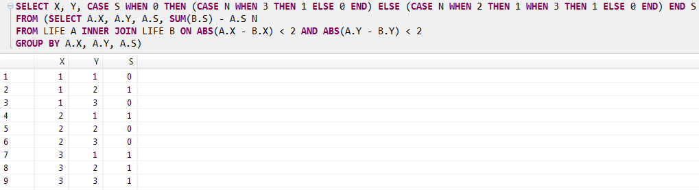
Based on the results of step 1, we apply the following simplified rules to calculate the next generation.
1) The current status of the cell is dead
If there are exactly three live neighbours, the next status will be live; Otherwise, the next status will be still dead.
2) The current status of the cell is live
If there are two or three live neighbours, the next status will be still live; Otherwise, the next status will be dead.
You can also check the results manually.

3. Update the "LIFE" table with the results in step 2
UPDATE LIFE SET S = NEXTGEN.S FROM LIFE,

(SELECT X, Y, CASE S WHEN 0 THEN (CASE N WHEN 3 THEN 1 ELSE 0 END) ELSE (CASE N WHEN 2 THEN 1 WHEN 3 THEN 1 ELSE 0 END) END S

FROM (SELECT A.X, A.Y, A.S, SUM(B.S) - A.S N

FROM LIFE A INNER JOIN LIFE B ON ABS(A.X - B.X) < 2 AND ABS(A.Y - B.Y) < 2

GROUP BY A.X, A.Y, A.S)) NEXTGEN

WHERE LIFE.X = NEXTGEN.X AND LIFE.Y = NEXTGEN.Y;
Perhaps you are not familiar with the special syntax of "UPDATE" here, don't worry. You can find the example at the bottom of UPDATE - SAP HANA SQL and System Views Reference - SAP Library. So far, we've created the first generation successfully.

You can repeat step 3 to play further. :wink:
Play with window function
If you think this is the end of the blog. You're wrong. What about play the game of life with window function in SAP HANA? As I mentioned in Window function vs. self-join in SAP HANA, if self-join exists in your SQL statement, please consider if it is possible to implement the logic with window function. Now let's play with window function. First of all, in order to compare with the self-join approach, we need to reset the "LIFE" table to the same initial pattern.

1. Calculate # of live neighbours for each cell
In the window function approach, we have two sub-steps as follows.
1) Calculate # of live "vertical" neighbours for each cell
SELECT X, Y, S, (S + IFNULL(LEAD(S) OVER (PARTITION BY X ORDER BY Y), 0) + IFNULL(LAG(S) OVER (PARTITION BY X ORDER BY Y), 0)) N FROM LIFE;

In this sub-step, we just calculate N(North) + C(Center) + S(South) for each C(Center). We partition the "LIFE" table by X vertically.
 from Moore neighborhood - Wikipedia
For instance, # of live "vertical" neighbours of cell (2, 2) is 2.

2) Calculate # of live neighbours for each cell
Based on sub-step 1), we can calculate the final result by partitioning the "LIFE" table horizontally. In this sub-step, we partition the table by Y.
SELECT X, Y, S, (N + IFNULL(LEAD(N) OVER (PARTITION BY Y ORDER BY X), 0) + IFNULL(LAG(N) OVER (PARTITION BY Y ORDER BY X), 0) - S) N

FROM (SELECT X, Y, S, (S + IFNULL(LEAD(S) OVER (PARTITION BY X ORDER BY Y), 0) + IFNULL(LAG(S) OVER (PARTITION BY X ORDER BY Y), 0)) N FROM LIFE);

Now we get the same result with the self-join approach.
2. Apply the rules to get the results of the next generation
SELECT X, Y, CASE S WHEN 0 THEN (CASE N WHEN 3 THEN 1 ELSE 0 END) ELSE (CASE N WHEN 2 THEN 1 WHEN 3 THEN 1 ELSE 0 END) END S

FROM (SELECT X, Y, S, (N + IFNULL(LEAD(N) OVER (PARTITION BY Y ORDER BY X), 0) + IFNULL(LAG(N) OVER (PARTITION BY Y ORDER BY X), 0) - S) N

FROM (SELECT X, Y, S, (S + IFNULL(LEAD(S) OVER (PARTITION BY X ORDER BY Y), 0) + IFNULL(LAG(S) OVER (PARTITION BY X ORDER BY Y), 0)) N FROM LIFE));

3. Update the "LIFE" table with the results in step 2
UPDATE LIFE SET S = NEXTGEN.S FROM LIFE,

(SELECT X, Y, CASE S WHEN 0 THEN (CASE N WHEN 3 THEN 1 ELSE 0 END) ELSE (CASE N WHEN 2 THEN 1 WHEN 3 THEN 1 ELSE 0 END) END S

FROM (SELECT X, Y, S, (N + IFNULL(LEAD(N) OVER (PARTITION BY Y ORDER BY X), 0) + IFNULL(LAG(N) OVER (PARTITION BY Y ORDER BY X), 0) - S) N

FROM (SELECT X, Y, S, (S + IFNULL(LEAD(S) OVER (PARTITION BY X ORDER BY Y), 0) + IFNULL(LAG(S) OVER (PARTITION BY X ORDER BY Y), 0)) N FROM LIFE))) NEXTGEN

WHERE LIFE.X = NEXTGEN.X AND LIFE.Y = NEXTGEN.Y;

Self-join vs. window function
Since we have only played the very small 3x3 game of life with SAP HANA, we cannot compare the performance between self-join and window function. In order to compare the performance, we need to generate a bigger grid. We can first create a stored procedure which enables us to generate a NxN grid.
CREATE PROCEDURE GENERATE_LIFE(IN X INTEGER) LANGUAGE SQLSCRIPT AS

i INTEGER;

j INTEGER;

BEGIN

  DELETE FROM LIFE;

  FOR i IN 1 .. X DO

  FOR j IN 1 .. X DO

  INSERT INTO LIFE VALUES (i, j, ROUND(RAND()));

  END FOR;

  END FOR;

END;
Then we can call the above stored procedure to generate the initial pattern, e.g., a 100x100 grid.
CALL GENERATE_LIFE(100);
Now let's do some comparisons. Here we just compare step 2 between self-join and window function since step 3 is just the update operation. Hence, we compare the following two SELECT statements.
Self-join
SELECT X, Y, CASE S WHEN 0 THEN (CASE N WHEN 3 THEN 1 ELSE 0 END) ELSE (CASE N WHEN 2 THEN 1 WHEN 3 THEN 1 ELSE 0 END) END S

FROM (SELECT A.X, A.Y, A.S, SUM(B.S) - A.S N

FROM LIFE A INNER JOIN LIFE B ON ABS(A.X - B.X) < 2 AND ABS(A.Y - B.Y) < 2

GROUP BY A.X, A.Y, A.S);
Window function
SELECT X, Y, CASE S WHEN 0 THEN (CASE N WHEN 3 THEN 1 ELSE 0 END) ELSE (CASE N WHEN 2 THEN 1 WHEN 3 THEN 1 ELSE 0 END) END S

FROM (SELECT X, Y, S, (N + IFNULL(LEAD(N) OVER (PARTITION BY Y ORDER BY X), 0) + IFNULL(LAG(N) OVER (PARTITION BY Y ORDER BY X), 0) - S) N

FROM (SELECT X, Y, S, (S + IFNULL(LEAD(S) OVER (PARTITION BY X ORDER BY Y), 0) + IFNULL(LAG(S) OVER (PARTITION BY X ORDER BY Y), 0)) N FROM LIFE));
Test environment:
- SAP HANA SPS08 Rev. 80
- CPU: 8 cores
- Memory: 64GB
- Disk: 200GB
| N = 100 | N = 400 | |
|---|---|---|
| # of cells | 100 * 100 = 10,000 | 400 * 400 = 160,000 |
| Time with self-join | ~40s | ~1400s |
| Time with window function | ~30ms | ~120ms |
From the above table, we can find the following results:
1. The performance of window function is much better than self-join.
2. The time with window function seems a linear function of N.
3. The time with self-join seems a exponential growth with N.
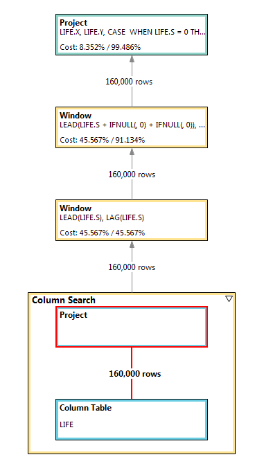
We can find some reasons from the following two visualization plans. It takes about 99.99% time for the large column search node in self-join to make the non equi join and do the filter. And the join result has 25,600,000,000 rows! Meanwhile, the visualization plan of window function shows that two sequential window nodes just need to consume # of cells.
Visualization plan of self-join (N = 400)

Visualization plan of window function (N = 400)
Conclusion
In this blog, we played the game of life with not only self-join but also window function in SAP HANA. From the results of comparison, we can find that if the grid is small, there is nearly no difference between the performance with self-join and window function. However, if we want to play a big game, it's highly recommended to play with window function instead of self-join; Otherwise, you'll lose the game... :sad:
Hope you enjoyed reading my blog. Have fun! :smile:
- SAP Managed Tags:
- SAP HANA
21 Comments
You must be a registered user to add a comment. If you've already registered, sign in. Otherwise, register and sign in.
Labels in this area
-
ABAP CDS Views - CDC (Change Data Capture)
2 -
AI
1 -
Analyze Workload Data
1 -
BTP
1 -
Business and IT Integration
2 -
Business application stu
1 -
Business Technology Platform
1 -
Business Trends
1,658 -
Business Trends
91 -
CAP
1 -
cf
1 -
Cloud Foundry
1 -
Confluent
1 -
Customer COE Basics and Fundamentals
1 -
Customer COE Latest and Greatest
3 -
Customer Data Browser app
1 -
Data Analysis Tool
1 -
data migration
1 -
data transfer
1 -
Datasphere
2 -
Event Information
1,400 -
Event Information
66 -
Expert
1 -
Expert Insights
177 -
Expert Insights
298 -
General
1 -
Google cloud
1 -
Google Next'24
1 -
Kafka
1 -
Life at SAP
780 -
Life at SAP
13 -
Migrate your Data App
1 -
MTA
1 -
Network Performance Analysis
1 -
NodeJS
1 -
PDF
1 -
POC
1 -
Product Updates
4,577 -
Product Updates
343 -
Replication Flow
1 -
RisewithSAP
1 -
SAP BTP
1 -
SAP BTP Cloud Foundry
1 -
SAP Cloud ALM
1 -
SAP Cloud Application Programming Model
1 -
SAP Datasphere
2 -
SAP S4HANA Cloud
1 -
SAP S4HANA Migration Cockpit
1 -
Technology Updates
6,873 -
Technology Updates
420 -
Workload Fluctuations
1
Related Content
- SAP Hana Calculation view input parameter from JPA Entity in Technology Q&A
- How to embed SWZ portal into an iFrame? in Technology Blogs by SAP
- HANA DB usage of JSON embedded functions in Technology Q&A
- CAP Autentication error in Technology Q&A
- LLM, RAG and Cloud Foundry: No space left on device in Technology Q&A
Top kudoed authors
| User | Count |
|---|---|
| 37 | |
| 25 | |
| 17 | |
| 13 | |
| 7 | |
| 7 | |
| 7 | |
| 6 | |
| 6 | |
| 6 |