
- SAP Community
- Products and Technology
- Technology
- Technology Blogs by SAP
- Introduction to R
Technology Blogs by SAP
Learn how to extend and personalize SAP applications. Follow the SAP technology blog for insights into SAP BTP, ABAP, SAP Analytics Cloud, SAP HANA, and more.
Turn on suggestions
Auto-suggest helps you quickly narrow down your search results by suggesting possible matches as you type.
Showing results for
Former Member
Options
- Subscribe to RSS Feed
- Mark as New
- Mark as Read
- Bookmark
- Subscribe
- Printer Friendly Page
- Report Inappropriate Content
07-16-2014
11:47 AM
This post is a beginner's guide on how to install R and run the first script. It is also a continuation of my previous post on One-to-One Marketing using Big Data and Predictive Analytics. But first things first, in case you are not already aware of what this beast is...
So, What is R?
R is a free statistical computing and graphics language and has been around for about 2 decades. The language continues to evolve with more functions added each day by the community. R's popularity stems from the numerous data manipulation and caluclation functions, and the depiction of the results using graphical display for easy data analysis. R is an interpreted language and can be accessed using a command-line interface.
I am not going into more details about R at present. My job here is to get you quickly acquainted, so R does not appear so formidable and mysterious anymore. I leave it to you to have lunch (or several lunches) together later and get to know R a lot better. Some suggested reading links for more information on R and what it is capable of:
Resources to help you learn and use R
Installing R and the IDE
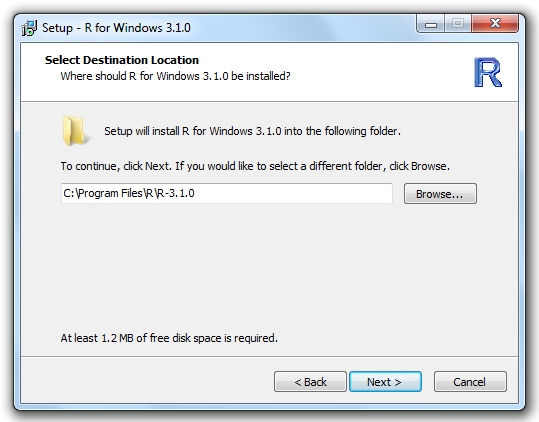
Right, back to the introduction! For the windows installation of the latest R release, please visit the link R 3.1.0 for Windows and download the software.
There are several IDEs in the market, but we are going with RStudio for our purposes. It is easy to install and use. You can download and install the version for Windows from this link RStudio 0.98.507. Click on the .exe file once downloaded:

You can set the destination folder of your choice, and choose the default options. That's it, nice and easy. We are ready to write our first R program.
Writing our first program in R
Launch the R studio to see a window like the one below:

You will find several datasets included in R packages which you can utilise. For the simple program below, I have used a dataset about players in the recently concluded football world cup (WC'14_Players.txt).
I have cleaned the data and extracted the information from the "Age" and "No. of Caps" columns to determine the correlation between them.
Type in the following statements in your console (the left bottom corner):
Age <- c(31,31,29,27,29,26,27,29,30,22,22,34,32,30,27,32,26,25,27,21,27,31,25,28,31,24,22,24,28,30,30,28,26,26,24,21,31,28,26,28,28,22,21,25,33,32,34,25,22,25,18,35,29,21,32,28,32,24,25,29,22,21,28,26,30,25,25,20,27,21,21,19,34,31,28,28,20,24,28,33,31,34,35,27,32,26,28,21,25,24,24,28,24,25,23,26,25,26,30,23,23,33,22,25,23,32,25,24,26,22,29,21,34,31,29,28,27,22,25,25,21,25,21,21,34,31,23,21,31,33,25,28,26,26,34,25,31,23,30,30,27,27,32,29,25,27,23,28,25,33,24,30,28,30,25,26,23,29,22,24,22,23,22,30,20,19,30,30,29,24,26,22,20,24,23,20,22,19,33,30,30,26,33,31,23,28,27,28,25,29,24,21,22,34,32,30,27,28,25,29,28,26,25,22,25,30,32,26,29,28,25,20,42,25,24,38,35,28,27,27,29,22,21,27,29,28,33,26,22,25,21,28,29,27,28,27,24,23,34,21,28,25,33,33,31,29,27,21,27,27,21,23,31,27,30,26,29,23,21,36,28,27,25,26,24,25,28,20,28,29,33,26,27,29,32,26,22,37,34,29,23,27,26,23,24,32,29,34,26,31,26,23,27,27,27,34,24,28,25,24,27,32,28,31,23,30,24,30,24,24,25,25,27,32,28,25,31,30,29,26,30,24,25,29,26,23,26,30,30,32,27,22,28,28,23,24,32,28,30,21,24,30,27,29,29,34,28,31,22,35,24,28,23,24,31,23,20,22,28,32,19,26,20,26,18,36,27,21,29,33,27,32,26,27,21,32,28,24,35,30,29,28,29,31,27,21,29,27,31,23,27,26,23,23,24,27,31,32,33,30,28,27,29,23,19,24,34,28,29,28,33,32,29,23,25,35,27,27,23,27,28,27,25,34,32,26,26,29,31,19,23,35,32,28,30,29,24,24,27,30,23,28,24,19,26,23,25,26,25,29,27,35,27,33,31,28,24,28,21,20,23,31,29,28,27,24,30,21,23,23,26,27,27,37,34,20,31,32,28,29,26,28,28,29,29,28,30,27,24,25,23,21,31,27,32,25,30,30,28,29,31,23,29,29,22,21,29,25,21,25,28,27,24,23,21,27,23,22,22,27,30,32,33,29,25,24,27,26,33,30,30,33,28,26,25,28,28,28,26,28,26,26,26,29,32,26,33,28,31,33,30,28,24,24,27,25,20,32,24,28,29,29,28,24,23,21,22,24,24,22,24,28,29,26,24,33,26,26,27,21,32,24,30,30,27,27,30,32,23,31,27,33,31,29,30,30,27,20,25,22,24,26,31,19,21,31,30,29,27,33,26,25,23,24,20,23,24,27,21,25,26,21,23,23,23,23,23,21,32,27,27,32,25,21,24,28,25,33,30,29,25,25,26,26,25,20,22,22,29,25,27,24,22,20,23,36,29,23,25,24,21,26,29,24,25,27,27,23,23,26,21,21,29,25,31,23,24,22,23,24,26,27,22,28,22,22,23,31,32,31,28,26,22,29,27,30,28,26,26,33,26,21,31,27,29,23,29,30,32,31,35,20,25,26,27,21,32,31,23,23,27,29,32,32,32,19,24,31,27,28,24,34,26,28,29,27,29,31,27,29,29,25,26,23,28,22,30,28,30,30,30,24,24,22,27,24,19,27,23,30,26,25,24,22,25,28,28,27,25,22,26,21,23,26,25,21,27,36,26,19,29,26,19,26,24,28,28,24,33,34,31,27,30,27,27,23,25,30,30,32,23,27,28,29,23,25,21,31,23,22,29,28,24,32,24,24,24,29,21,28,29,27,25,24,25,25,25,26,23,24,23,21,25)
Caps <- c(9,73,45,34,6,29,41,23,31,47,29,78,70,11,4,7,17,25,33,10,15,6,5,12,7,2,0,45,30,29,20,14,11,7,5,2,66,48,44,38,35,20,7,2,115,54,38,24,22,14,6,109,6,0,111,71,48,23,22,20,5,2,73,60,54,27,9,8,4,0,0,0,90,62,48,32,3,0,57,33,13,120,118,101,92,50,28,13,12,14,12,11,10,7,6,2,73,59,31,23,4,8,6,3,1,80,17,9,8,6,2,0,73,46,43,28,22,14,13,10,9,3,1,1,68,34,7,4,78,7,4,64,59,45,28,23,18,1,58,56,53,42,28,22,19,19,16,11,65,34,28,25,24,14,6,5,0,22,14,14,10,2,2,2,1,1,97,73,69,10,9,8,5,5,4,1,1,0,98,83,61,20,153,30,0,115,59,45,25,6,5,2,0,130,109,94,87,78,63,61,34,31,15,7,0,106,94,37,23,20,1,0,54,42,0,95,75,51,50,20,12,4,1,48,47,43,29,26,21,8,3,51,28,26,23,9,7,5,79,1,1,0,119,106,78,42,18,8,3,3,0,0,83,43,25,24,5,2,0,99,64,53,24,20,7,6,17,1,1,64,47,46,28,20,16,12,6,132,109,47,16,16,14,4,3,73,71,69,29,55,66,12,54,68,8,142,25,74,55,10,12,55,4,79,10,78,7,20,4,16,39,2,51,20,4,2,81,60,47,33,25,24,10,2,2,1,61,53,42,39,33,21,16,11,9,0,93,61,37,31,22,17,39,50,22,109,23,24,15,103,10,89,21,10,6,8,14,9,45,4,2,3,3,1,1,139,7,0,67,47,35,33,12,11,9,3,1,0,108,93,57,41,33,19,19,4,2,0,35,29,29,10,4,4,1,60,4,0,92,88,76,55,41,13,4,2,88,71,61,55,54,53,42,27,25,108,77,60,11,8,23,18,3,88,57,36,35,21,21,2,0,108,80,69,48,41,38,28,20,18,17,10,7,1,0,0,48,29,8,1,55,11,2,55,39,20,17,16,5,2,2,81,32,28,21,15,10,9,4,2,65,28,23,120,25,0,102,75,66,52,31,20,9,92,92,46,39,39,34,20,18,15,68,41,21,10,55,61,34,52,40,5,73,71,9,24,46,5,19,22,32,46,10,19,5,43,0,5,31,45,10,3,37,36,24,20,18,16,13,8,96,53,47,45,24,19,16,7,5,5,84,50,36,29,15,28,3,0,0,72,22,12,11,7,6,5,2,80,46,41,40,34,33,20,10,7,5,3,1,1,0,60,53,9,8,11,5,3,2,0,84,60,48,22,20,19,17,16,6,5,5,138,78,59,49,15,12,6,6,3,40,12,6,1,1,89,32,11,0,95,41,35,34,32,16,10,9,58,34,21,21,19,19,13,12,12,11,1,59,48,21,6,5,3,2,45,2,1,105,96,37,28,19,16,4,2,1,0,101,53,44,42,27,11,1,131,112,31,19,47,1,20,17,6,45,39,29,25,16,8,5,1,81,60,56,48,47,21,16,15,13,11,3,78,11,11,0,32,70,57,46,43,2,110,66,53,6,6,29,16,6,1,73,72,21,2,10,34,6,66,98,3,19,84,15,3,115,103,8,18,27,24,40,15,35,1,68,20,21,25,11,14,20,27,6,5,1,61,27,25,24,12,6,5,4,1,28,27,24,23,22,17,16,9,6,4,1,1,0,33,20,18,4,15,33,48,58,56,46,21,49,28,44,44,14,0,23,78,43,1,26,55,1,25,19,8,67,2,1,95,76,21,10,9,4,3,0,60,42,41,31,25,17,15,5,4,1,79,20,1,60,8,3,34,20,3,27,13,24,63,63,11,36,9,10,57,54,26,27,24,5,10,0)
plot(Age,Caps)
cor.test(Age,Caps,alternative = "g")
The first statement assigns an array of integer values (the ages of all the players) to a variable Age.
The second statement assigns an array of integer values (the no. of times the players have been capped) to a variable Caps.
The third statement (plot(Age,Caps)) draws an output scatter plot diagram in the right bottom corner.
The fourth statement (cor.test(Age,Caps,alternative = "g")) determines the correlation between the two variables.
The output looks like this:

A positive correlation of 0.6025268 is indicated. While the correlation is not very strong, it definitely confirms that older players have been capped more no. of times for their country.
In the next blog post, I shall explore some of the following data mining techniques by utilizing the R integration for SAP HANA:
- Cluster Analysis
- Regression Analysis
- Association Analysis
- Classification Analysis
- Time Series Analysis
- Multivariate Statistics
- Analysis of Spatial Data
- SAP Managed Tags:
- SAP Predictive Analytics,
- Careers
You must be a registered user to add a comment. If you've already registered, sign in. Otherwise, register and sign in.
Labels in this area
-
ABAP CDS Views - CDC (Change Data Capture)
2 -
AI
1 -
Analyze Workload Data
1 -
BTP
1 -
Business and IT Integration
2 -
Business application stu
1 -
Business Technology Platform
1 -
Business Trends
1,658 -
Business Trends
91 -
CAP
1 -
cf
1 -
Cloud Foundry
1 -
Confluent
1 -
Customer COE Basics and Fundamentals
1 -
Customer COE Latest and Greatest
3 -
Customer Data Browser app
1 -
Data Analysis Tool
1 -
data migration
1 -
data transfer
1 -
Datasphere
2 -
Event Information
1,400 -
Event Information
66 -
Expert
1 -
Expert Insights
177 -
Expert Insights
297 -
General
1 -
Google cloud
1 -
Google Next'24
1 -
Kafka
1 -
Life at SAP
780 -
Life at SAP
13 -
Migrate your Data App
1 -
MTA
1 -
Network Performance Analysis
1 -
NodeJS
1 -
PDF
1 -
POC
1 -
Product Updates
4,577 -
Product Updates
343 -
Replication Flow
1 -
RisewithSAP
1 -
SAP BTP
1 -
SAP BTP Cloud Foundry
1 -
SAP Cloud ALM
1 -
SAP Cloud Application Programming Model
1 -
SAP Datasphere
2 -
SAP S4HANA Cloud
1 -
SAP S4HANA Migration Cockpit
1 -
Technology Updates
6,873 -
Technology Updates
420 -
Workload Fluctuations
1
Related Content
- Customer & Partner Roundtable for SAP BTP ABAP Environment #12 in Technology Blogs by SAP
- Consuming SAP with SAP Build Apps - Mobile Apps for iOS and Android in Technology Blogs by SAP
- Composite Data Source Configuration in Optimized Story Experience in Technology Blogs by SAP
- QM Notification Configuration from DMC to ERP in Technology Blogs by Members
- Exploring Integration Options in SAP Datasphere with the focus on using SAP extractors - Part II in Technology Blogs by SAP
Top kudoed authors
| User | Count |
|---|---|
| 37 | |
| 25 | |
| 17 | |
| 13 | |
| 7 | |
| 7 | |
| 7 | |
| 6 | |
| 6 | |
| 6 |