
- SAP Community
- Products and Technology
- Technology
- Technology Blogs by Members
- Thinking in HANA - Part 2: Revisiting SCDs
Technology Blogs by Members
Explore a vibrant mix of technical expertise, industry insights, and tech buzz in member blogs covering SAP products, technology, and events. Get in the mix!
Turn on suggestions
Auto-suggest helps you quickly narrow down your search results by suggesting possible matches as you type.
Showing results for
Former Member
Options
- Subscribe to RSS Feed
- Mark as New
- Mark as Read
- Bookmark
- Subscribe
- Printer Friendly Page
- Report Inappropriate Content
03-24-2014
1:58 AM
Hi again folks,
It's been a few weeks since my first post in my series "Thinking on HANA", so I think it's about time for me to get the next article written up, posted, discussed, debated, critiqued, printed, turned into paper airplanes...
For those of you who have been following my posts over the past year or so, it's hopefully clear by now that one of the themes of my work is, "there's more than one way to skin a cat. I stated this a bit more formally in my last post,
As a massively-parallel, column-oriented, in-memory platform, HANA affords many opportunities to come up with new and creative solutions to seemingly well-understood problems.
In addition to exploring technical aspects of alternative solutions, I'd also like to start framing these alternatives in the bigger picture of "organizational problem-solving" (okay - "consulting") where, in addition to technical trade-offs, organizational-imposed constraints restrict the solution domain even further. The stereotypical example in IT (and other fields) is the "triple constraint" in Project Management of time, cost and quality - the three resource constraints of all organizational projects. This "triple constraint" is, of course, only a heuristic to help guide project management decision-making. Constraints such as risks, financial costs, environmental costs, social costs, scope, performance, etc can be mapped to any number of "focal points" that make the most sense (heaven forbid we start talking about hierarchies of constraints!)
When developing solutions on HANA, and more specifically, during the phase in which I research, consider and prototype as many data modeling solutions as are feasible, I typically characterize the solution set with the following model:

Functionality
- Does the solution meet the ad-hoc requirements? Visualization requirements?
- Does it support the data structure requirements? (i.e. hierarchy for MDX clients)
- Does it provide the required result set?
Performance
- Do queries execute sufficiently fast?
- Are there any concerns regarding memory consumption?
Maintainability
- Is the solution well-understood by other practitioners?
- Can it be easily maintained?
Velocity
- Does the solution meet the real-time and/or batch requirements from source system to HANA?
Resources
- Can the solution be implemented in a reasonable amount of time and cost given available resources?
As should be immediately obvious, these constraints can easily be mapped to the classic project management "triple constraint", and with a bit of "refactoring" could certainly fit into four or six or N number of discrete concerns.
Keeping in mind these constraints, let's evaluate 5 different solutions to modeling "slowly changing dimensions” (SCDs) in HANA.
Slowly Changing Dimensions
I characterize slowly-changing dimensions as those attributes of “organizational entities” that 1) change over time and 2) have an impact on business processes that can and likely should be measured to assist in organizational decision-making. (For all the messy details free to reference Wikipedia's treatise on all 6+ different types). Generally these attributes are lost in transactional systems (i.e. they are treated like CRUD – created, read, updated, deleted – but not maintained or tracked over time).
Let’s take a very simple example that illustrates the concept.
Imagine a product that goes through a typical technology lifecycle – it’s built with one metal and over time upgraded with lighter and stronger metals (okay, carbon fiber isn't a metal, fair enough). Below shows an image of material changes over time – within the single month of January (I know, not very realistic, use your imagination ).

This data can be captured with the following table structure:

PROD_ID is the primary key of the product, DATE_FROM and DATE_TO capture the “validity period” of the material attribute, and MATERIAL captures the physical material the product is made of during that period.
Next, imagine this product is sold throughout all of January. Again, for simplicity’s sake – we’ll use an *incredibly* simple model. In our alternate universe here, a single sale for $100 was registered in every day of January for the product. No additional information was captured. (Imaginations, people!). Here is the table structure. It should be self-explanatory. TX_DATE is the transaction date.

Although the example already speaks for itself, let’s assume we want to analyze the aggregate sales for the product for each material that it was made out of. We would accomplish this by joining the two tables on PROD_ID as well as joining the tables where the transaction date (TX_DATE) of the sales table falls between the validity dates (DATE_FROM and DATE_TO) of the product material table. What’s also important is that we analyze sales for those days where we mistakenly didn’t track the product’s material – we still want to see the sales for those products.
Following are five alternative solutions that I'll describe for modeling slowly-changing dimensions in HANA:
- Theta Join #1
- Theta Join #2
- SQLScript
- Temporal Join
- Surrogate Key
I’ll demonstrate each approach, follow each with a discussion on the pros and cons with respect to the constraints provided earlier, and I’ll end this article with a bird’s eye view on the implications for these kinds of requirements and solutions.
Theta Join #1
I use the term “thetajoin” to describe any join condition that is somewhere between the “natural” join conditions (i.e. those which respect the cardinality of the relationship between the tables) and a “cross join”, otherwise called a Cartesian product, which maps every record in one table to reach record in the other table.
For those who are interested in the precise definitions of terms like “theta join”, a simple google search should serve you well. Hopefully I don’t upset folks too much by being a bit liberal/imprecise with my use of these terms.
In the screenshot below, you’ll see that the sales table and the material table are only joined on PROD_ID.

The conditional component of the join is handled in the following calculated column, where the logic only populates the column with the sales amount if it finds that the transaction date falls between the beginning and end dates of the validity period.

Querying the data model for validity dates, material and amounts gives the following result.

Let’s discuss the data model and the results in the context of the constraints discussed initially.
Functionality
This approach solves the main requirement – aggregating sales per material type – but fails to pull through any sales figures that don’t correspond to material values (i.e. where material is null). In order to achieve this final requirement, the model would actually have to output calculated attribute values per validity period – basically the same calculation but for the dimensions rather than the single measure. The base measure should then come through alone, and when grouped by calculated dimensions, it would effectively display the final result with an additional record with nulls in the other columns as expected.
Maintainability
The model above is relatively straightforward to understand. However, it’s deceiving. The left outer join implies to the developer that all fact records will be captured as is the case with most data models – but the condition of the calculated measure renders this characteristic void. Moreover, the “theta join” is not particularly intuitive. Also, if the solution was implemented with calculated attributes instead of the calculated measure – as described above, which would give 100% correct functional results – this kind of approach would be entirely unsustainable. The amount of work (in production situation, tens or hundreds of calculated attributes), the confusion of the approach, the room for error, and the performance implications would make this a very bad decision.
Velocity
This approach can be modeled against real-time (i.e. SLT sourced) or batched (i.e. ETL sourced) data if source data has validity periods. If source data does not have validity periods, an ETL job will have to capture the validity periods. If SLT is used, an approach like this one should be used to capture validity periods.
Resources
This approach should be pretty quick to develop without taxing the development team too heavily. SLT-sourced data, however, will require additional resources to implement the history-tracking approach referenced above if this is pursued.
Performance
This model will first execute in the OLAP engine, and the aggregated results will be processed by the Calculation Engine for the calculated measure to arrive at the final result. Since both engines are required to process the result, performance will suffer. Moreover, extra memory will be consumed to accommodate the theta join (which results in more intermediate records before final result set is built).
Theta Join #2
The following approach is similar to the first one. In the analytic view, the only join condition modeled is the equijoin on PROD_ID between the two tables.
However, the conditional logic is implemented as a filter in a projection node with a Calculation View, and the base measure is pulled through.

Following are the results:

Functionality
This approach suffers from the same shortcoming as the first – any fact records that don’t have corresponding dimensions are effectively dropped from the result set.
Maintainability
The approach is about as maintainable as the first one.
Velocity
As is the case previously, this approach will support realtimeor batched data – with the requirement that the tables have validity periods. Extra logic may need to implemented in the ETL layer or SLT (or other replication layer) to capture validity periods if source tables are not already populated with them
Resources
This model has about the same development resource requirements as the first model.
Performance
This model will perhaps perform slightly better than the first. In my experience, computations are more expensive than filters. The theta join poses the same risk of additional memory consumption.
SQLScript
Below is SQLScript syntax of a scripted Calculation View that captures the traditional SQL syntax used to join slowly changing dimensions to fact tables.

Following are the results of the model:

Functionality
This approach gives 100% correct functional results.
Maintainability
Modeling slowly changing dimensions via SQLScript is not very maintainable. All SCD tables must be modeled in SQLScript, an output table with correct field names, data types, potentially capitalization and ordering must be maintained.
Velocity
As is the case previously, this approach will support realtime or batched data – with the requirement that the tables have validity periods. Extra logic may need to implemented in the ETL layer or SLT (or other replication layer) to capture validity periods if source tables are not already populated with them.
Resources
Developing this model requires strong SQL skills in developer resources. The scripted nature of the approach will also take more time to develop and debug than a graphical approach.
Performance
This model will likely have bad performance. Depending on the granularity of the dimension in the fact table, the OLAP Engine* will execute limited aggregation before handing off a large intermediate resultset to the SQL Engine to process the SCD component (which will never be pruned and thus always executed). Moreover, only equijoins are natively support in the column store – which can be examined with a VizPlan analysis against this model. As noted, the join cannot be handled by a column scan (i.e. one of HANA’s fundamental strengths) and thus will be slow to execute:
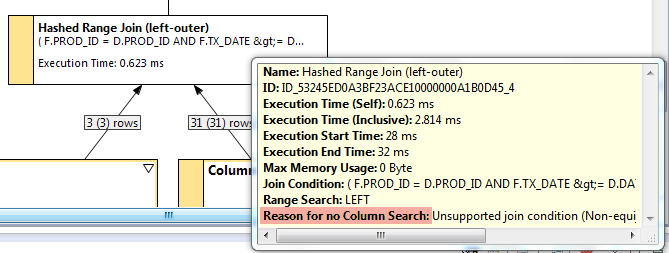
*the example above was built against raw tables, but in real-life scenarios it would likely be built against analytic views.
Temporal Join
HANA’s native feature for modeling slowly changing dimensions is called a “temporal join” and is modeled within an Analytic View is shown below:

As you can see, the join condition is specified both by the graphical equijoin as well as the temporal conditions listed in the Properties tab of the join.
Following are the results:

Functionality
This modeling approach suffers from the same fate as the first two models of this article – fact records that lack corresponding dimensions are dropped. This is due to the fact that the temporal join can only be modeled against Referential join types – which effectively function as inner joins when the respective dimensions are included in the query. This is a significant drawback to the temporal join.
Maintainability
HANA’s Temporal Join was slated to be the native solution to modeling slowly changing dimensions. As such, it’s well-documented, taught, and understood. It’s easy to model and is available directly in Analytic Views, making it very maintainable.
Velocity
As is the case previously, this approach will support realtime or batched data – with the requirement that the tables have validity periods. Extra logic may need to implemented in the ETL layer or SLT (or other replication layer) to capture validity periods if source tables are not already populated with them.
Resources
No additional resources from a development perspective are required for this approach, aside from those that may be required for implementing validity period capture in ETL or replication layer of the landscape.
Performance
In my experience, temporal joins execute with similar performance as other join types. (I have not done extensive testing with this approach, however, as I have not yet worked on a project where either the data was “referentially complete”, or where the customer was willing to accept an incomplete result set.) I’d be curious to learn more about how the temporal join actually works. The VizPlan shows a Column Search for the join as with typical models, but no additional “helper” columns (like compound join concatenated columns) were found in M_CS_ALL_COLUMNS. As such, I’m not exactly sure how the temporal aspect of the join is handled.
Surrogate Key
The final modeling approach provided is well-represented in the world of data warehousing. Tables with slowly changing dimensions are populated with a generated (“surrogate”) key that is unique per combination of natural key fields and validity period. Then, the fact table is similarly populated for records whose natural key fields correspond with the dimension and whose transaction date falls between the respective dimension record’s validity dates. Any fact records that don’t have corresponding dimensions are typically populated with a value of -1 for the surrogate key.
The screenshot below shows this approach:

Here are the results:
Functionality
This modeling approach gives 100% correct results.
Maintainability
A simple equijoin in an Analytic View is likely the most well understood modeling approach in HANA. It involves nothing more than a graphical connection and a few property specifications. No coding or detailed maintenance is required. As such, this approach is very maintainable.
Velocity
In a traditional landscape, this approach will only support batched data where surrogate key population is handled by a scheduled ETL job. In theory, careful use of triggers could handle surrogate key population against replicated data, but I’ve never tried this in practice. The maintainability and performance implications may be prohibitive.
Resources
An ETL developer will need to build the logic for surrogate key population.
Performance
This approach will give the best performance as the equijoin condition is natively supported by HANA’s OLAP Engine. Moreover, if no dimension fields are included in the client query – or even if the join field is included – HANA will prune the join off from query execution – resulting in better performance.
Discussion
In the introduction to this post, I highlighted a shared theme between this post and the first one in my “Thinking in HANA” series, pointing out that HANA may offer multiple compelling solutions to the same problem.
I can also slightly modify another point made in “Thinking in HANA: Part 1” and find wide applicability to the issues raised when modeling slowly changing dimensions in HANA:
- Complex data flows captured in hand-coded SQL and/or SQLScript can be difficult to maintain.
- SQL queries against raw tables, whether hand-coded or software-generated (i.e. from a semantic layer like BOBJ Universes), often fail to leverage native high-performance engines in HANA (i.e. OLAP/Calc Engine).
- ...
- Some SQL operators can't be modeled in HANA a 1:1 fashion. For example, the SQL BETWEEN condition is limited in how it can be natively modeled in HANA.
Some readers of this article are probably left with at least the following two questions, if not more:
- Why don’t you show any performance metrics for the different approaches?
- Which approach would you recommend as the best?
Here are my answers:
- In short, I don’t currently have datasets on any current projects that I can leverage to do performance testing. We’re in the process of building ETL jobs to populate surrogate keys on a single conformed dimension table for HR data, but it will be another week or two until this is complete and I didn’t want to delay this post any longer.
- Even though I just now mentioned that we’re using the ETL approach to populate surrogate keys in order to model SCDs for our project, I can’t recommend this approach across the board. The best answer I can give for what you should do is the same answer given by all the computer science sages across the ages – “it depends”.
Are you building a one-off data model for a very small use case against tables that already have validity periods but lack referential integrity? I don’t see too much harm in going with the SQL approach.
Are you building a large-scale solution that needs to have the best performance possible and support a consistent enterprise-wide data architecture with limited real-time data velocity requirements? Then go with the ETL approach.
Does your client have a dashboarding need where only metrics plotted against actual dimensions are required? Perhaps one of the “theta-join” approaches is right for you.
Are you simply missing “blank” records in your dimension tables which are hindering referential integrity required for temporal join functional correctness? First implement this clever solution by justin.molenaur2 and you’ll be right as rain with the temporal join.
However, the point of this article is to equip you with a few “yardsticks” that you can use to help discern what the best approach is based on your specific technical, organizational (and dare I say SLA) constraints.
Final Thoughts
The more time one spends working on HANA, the more one begins to realize how many options are available. Just take a simple piece of conditional logic, for example, like that found in the join condition of SCDs. No matter where the logic is specified in a functional requirements document, it’s quite possible that that logic could be built into any of:
- a calculated measure (the first approach)
- a calculated attribute (mentioned in the first approach)
- a CalcView’s projection node filter (second approach)
- a SQLScript “node” (third approach)
- a HANA temporal join (fourth approach)
- persisted columns (fifth approach)
- semantic-layer generated SQL (not discussed here)
And those are just for the “class” of conditional logic found in joins. Depending on requirements, conditional logic (again, almost the simplest requirement one can boil any logic down to) could also be built into:
- generated columns in HANA (persisted)
- SLT (persisted)
- Restricted measures (on-the-fly)
- Set operations (i.e. replacing “or” conditions in joins or calculations with UNION ALL set operators between two “halves” of the original dataset – a particularly easy and effective performance tuning solution )
- Triggers (persisted)
- Many more places I’m sure I haven’t thought of!
As the old adage goes, “When the only thing you have is a hammer, everything begins to look like a nail.” Often times new consultants coming fresh out of HA300 will see the HANA world in terms of simple Attribute/Analytic/Calculation Views, when in reality, HANA offers a wealth of technology and innovation even on some of the simplest, most well-understood problems.
Take the time to understand the technical landscape, the true business requirements and constraints, and the multitude ways that business problems can be solved on HANA – and you’ll be well positioned to deliver high-performing world-class HANA solutions for your clients.
- SAP Managed Tags:
- SAP HANA
13 Comments
You must be a registered user to add a comment. If you've already registered, sign in. Otherwise, register and sign in.
Labels in this area
-
"automatische backups"
1 -
"regelmäßige sicherung"
1 -
"TypeScript" "Development" "FeedBack"
1 -
505 Technology Updates 53
1 -
ABAP
14 -
ABAP API
1 -
ABAP CDS Views
2 -
ABAP CDS Views - BW Extraction
1 -
ABAP CDS Views - CDC (Change Data Capture)
1 -
ABAP class
2 -
ABAP Cloud
2 -
ABAP Development
5 -
ABAP in Eclipse
1 -
ABAP Platform Trial
1 -
ABAP Programming
2 -
abap technical
1 -
absl
2 -
access data from SAP Datasphere directly from Snowflake
1 -
Access data from SAP datasphere to Qliksense
1 -
Accrual
1 -
action
1 -
adapter modules
1 -
Addon
1 -
Adobe Document Services
1 -
ADS
1 -
ADS Config
1 -
ADS with ABAP
1 -
ADS with Java
1 -
ADT
2 -
Advance Shipping and Receiving
1 -
Advanced Event Mesh
3 -
AEM
1 -
AI
7 -
AI Launchpad
1 -
AI Projects
1 -
AIML
9 -
Alert in Sap analytical cloud
1 -
Amazon S3
1 -
Analytical Dataset
1 -
Analytical Model
1 -
Analytics
1 -
Analyze Workload Data
1 -
annotations
1 -
API
1 -
API and Integration
3 -
API Call
2 -
Application Architecture
1 -
Application Development
5 -
Application Development for SAP HANA Cloud
3 -
Applications and Business Processes (AP)
1 -
Artificial Intelligence
1 -
Artificial Intelligence (AI)
5 -
Artificial Intelligence (AI) 1 Business Trends 363 Business Trends 8 Digital Transformation with Cloud ERP (DT) 1 Event Information 462 Event Information 15 Expert Insights 114 Expert Insights 76 Life at SAP 418 Life at SAP 1 Product Updates 4
1 -
Artificial Intelligence (AI) blockchain Data & Analytics
1 -
Artificial Intelligence (AI) blockchain Data & Analytics Intelligent Enterprise
1 -
Artificial Intelligence (AI) blockchain Data & Analytics Intelligent Enterprise Oil Gas IoT Exploration Production
1 -
Artificial Intelligence (AI) blockchain Data & Analytics Intelligent Enterprise sustainability responsibility esg social compliance cybersecurity risk
1 -
ASE
1 -
ASR
2 -
ASUG
1 -
Attachments
1 -
Authorisations
1 -
Automating Processes
1 -
Automation
2 -
aws
2 -
Azure
1 -
Azure AI Studio
1 -
B2B Integration
1 -
Backorder Processing
1 -
Backup
1 -
Backup and Recovery
1 -
Backup schedule
1 -
BADI_MATERIAL_CHECK error message
1 -
Bank
1 -
BAS
1 -
basis
2 -
Basis Monitoring & Tcodes with Key notes
2 -
Batch Management
1 -
BDC
1 -
Best Practice
1 -
bitcoin
1 -
Blockchain
3 -
bodl
1 -
BOP in aATP
1 -
BOP Segments
1 -
BOP Strategies
1 -
BOP Variant
1 -
BPC
1 -
BPC LIVE
1 -
BTP
12 -
BTP Destination
2 -
Business AI
1 -
Business and IT Integration
1 -
Business application stu
1 -
Business Application Studio
1 -
Business Architecture
1 -
Business Communication Services
1 -
Business Continuity
1 -
Business Data Fabric
3 -
Business Partner
12 -
Business Partner Master Data
10 -
Business Technology Platform
2 -
Business Trends
4 -
CA
1 -
calculation view
1 -
CAP
3 -
Capgemini
1 -
CAPM
1 -
Catalyst for Efficiency: Revolutionizing SAP Integration Suite with Artificial Intelligence (AI) and
1 -
CCMS
2 -
CDQ
12 -
CDS
2 -
Cental Finance
1 -
Certificates
1 -
CFL
1 -
Change Management
1 -
chatbot
1 -
chatgpt
3 -
CL_SALV_TABLE
2 -
Class Runner
1 -
Classrunner
1 -
Cloud ALM Monitoring
1 -
Cloud ALM Operations
1 -
cloud connector
1 -
Cloud Extensibility
1 -
Cloud Foundry
4 -
Cloud Integration
6 -
Cloud Platform Integration
2 -
cloudalm
1 -
communication
1 -
Compensation Information Management
1 -
Compensation Management
1 -
Compliance
1 -
Compound Employee API
1 -
Configuration
1 -
Connectors
1 -
Consolidation Extension for SAP Analytics Cloud
2 -
Control Indicators.
1 -
Controller-Service-Repository pattern
1 -
Conversion
1 -
Cosine similarity
1 -
cryptocurrency
1 -
CSI
1 -
ctms
1 -
Custom chatbot
3 -
Custom Destination Service
1 -
custom fields
1 -
Customer Experience
1 -
Customer Journey
1 -
Customizing
1 -
cyber security
3 -
Data
1 -
Data & Analytics
1 -
Data Aging
1 -
Data Analytics
2 -
Data and Analytics (DA)
1 -
Data Archiving
1 -
Data Back-up
1 -
Data Governance
5 -
Data Integration
2 -
Data Quality
12 -
Data Quality Management
12 -
Data Synchronization
1 -
data transfer
1 -
Data Unleashed
1 -
Data Value
8 -
database tables
1 -
Datasphere
2 -
datenbanksicherung
1 -
dba cockpit
1 -
dbacockpit
1 -
Debugging
2 -
Delimiting Pay Components
1 -
Delta Integrations
1 -
Destination
3 -
Destination Service
1 -
Developer extensibility
1 -
Developing with SAP Integration Suite
1 -
Devops
1 -
digital transformation
1 -
Documentation
1 -
Dot Product
1 -
DQM
1 -
dump database
1 -
dump transaction
1 -
e-Invoice
1 -
E4H Conversion
1 -
Eclipse ADT ABAP Development Tools
2 -
edoc
1 -
edocument
1 -
ELA
1 -
Embedded Consolidation
1 -
Embedding
1 -
Embeddings
1 -
Employee Central
1 -
Employee Central Payroll
1 -
Employee Central Time Off
1 -
Employee Information
1 -
Employee Rehires
1 -
Enable Now
1 -
Enable now manager
1 -
endpoint
1 -
Enhancement Request
1 -
Enterprise Architecture
1 -
ETL Business Analytics with SAP Signavio
1 -
Euclidean distance
1 -
Event Dates
1 -
Event Driven Architecture
1 -
Event Mesh
2 -
Event Reason
1 -
EventBasedIntegration
1 -
EWM
1 -
EWM Outbound configuration
1 -
EWM-TM-Integration
1 -
Existing Event Changes
1 -
Expand
1 -
Expert
2 -
Expert Insights
2 -
Fiori
14 -
Fiori Elements
2 -
Fiori SAPUI5
12 -
Flask
1 -
Full Stack
8 -
Funds Management
1 -
General
1 -
General Splitter
1 -
Generative AI
1 -
Getting Started
1 -
GitHub
8 -
Grants Management
1 -
groovy
1 -
GTP
1 -
HANA
6 -
HANA Cloud
2 -
Hana Cloud Database Integration
2 -
HANA DB
2 -
HANA XS Advanced
1 -
Historical Events
1 -
home labs
1 -
HowTo
1 -
HR Data Management
1 -
html5
8 -
HTML5 Application
1 -
Identity cards validation
1 -
idm
1 -
Implementation
1 -
input parameter
1 -
instant payments
1 -
Integration
3 -
Integration Advisor
1 -
Integration Architecture
1 -
Integration Center
1 -
Integration Suite
1 -
intelligent enterprise
1 -
iot
1 -
Java
1 -
job
1 -
Job Information Changes
1 -
Job-Related Events
1 -
Job_Event_Information
1 -
joule
4 -
Journal Entries
1 -
Just Ask
1 -
Kerberos for ABAP
8 -
Kerberos for JAVA
8 -
KNN
1 -
Launch Wizard
1 -
Learning Content
2 -
Life at SAP
5 -
lightning
1 -
Linear Regression SAP HANA Cloud
1 -
local tax regulations
1 -
LP
1 -
Machine Learning
2 -
Marketing
1 -
Master Data
3 -
Master Data Management
14 -
Maxdb
2 -
MDG
1 -
MDGM
1 -
MDM
1 -
Message box.
1 -
Messages on RF Device
1 -
Microservices Architecture
1 -
Microsoft Universal Print
1 -
Middleware Solutions
1 -
Migration
5 -
ML Model Development
1 -
Modeling in SAP HANA Cloud
8 -
Monitoring
3 -
MTA
1 -
Multi-Record Scenarios
1 -
Multiple Event Triggers
1 -
Neo
1 -
New Event Creation
1 -
New Feature
1 -
Newcomer
1 -
NodeJS
2 -
ODATA
2 -
OData APIs
1 -
odatav2
1 -
ODATAV4
1 -
ODBC
1 -
ODBC Connection
1 -
Onpremise
1 -
open source
2 -
OpenAI API
1 -
Oracle
1 -
PaPM
1 -
PaPM Dynamic Data Copy through Writer function
1 -
PaPM Remote Call
1 -
PAS-C01
1 -
Pay Component Management
1 -
PGP
1 -
Pickle
1 -
PLANNING ARCHITECTURE
1 -
Popup in Sap analytical cloud
1 -
PostgrSQL
1 -
POSTMAN
1 -
Process Automation
2 -
Product Updates
4 -
PSM
1 -
Public Cloud
1 -
Python
4 -
Qlik
1 -
Qualtrics
1 -
RAP
3 -
RAP BO
2 -
Record Deletion
1 -
Recovery
1 -
recurring payments
1 -
redeply
1 -
Release
1 -
Remote Consumption Model
1 -
Replication Flows
1 -
research
1 -
Resilience
1 -
REST
1 -
REST API
1 -
Retagging Required
1 -
Risk
1 -
Rolling Kernel Switch
1 -
route
1 -
rules
1 -
S4 HANA
1 -
S4 HANA Cloud
1 -
S4 HANA On-Premise
1 -
S4HANA
3 -
S4HANA_OP_2023
2 -
SAC
10 -
SAC PLANNING
9 -
SAP
4 -
SAP ABAP
1 -
SAP Advanced Event Mesh
1 -
SAP AI Core
8 -
SAP AI Launchpad
8 -
SAP Analytic Cloud Compass
1 -
Sap Analytical Cloud
1 -
SAP Analytics Cloud
4 -
SAP Analytics Cloud for Consolidation
3 -
SAP Analytics Cloud Story
1 -
SAP analytics clouds
1 -
SAP BAS
1 -
SAP Basis
6 -
SAP BODS
1 -
SAP BODS certification.
1 -
SAP BTP
21 -
SAP BTP Build Work Zone
2 -
SAP BTP Cloud Foundry
6 -
SAP BTP Costing
1 -
SAP BTP CTMS
1 -
SAP BTP Innovation
1 -
SAP BTP Migration Tool
1 -
SAP BTP SDK IOS
1 -
SAP Build
11 -
SAP Build App
1 -
SAP Build apps
1 -
SAP Build CodeJam
1 -
SAP Build Process Automation
3 -
SAP Build work zone
10 -
SAP Business Objects Platform
1 -
SAP Business Technology
2 -
SAP Business Technology Platform (XP)
1 -
sap bw
1 -
SAP CAP
2 -
SAP CDC
1 -
SAP CDP
1 -
SAP CDS VIEW
1 -
SAP Certification
1 -
SAP Cloud ALM
4 -
SAP Cloud Application Programming Model
1 -
SAP Cloud Integration for Data Services
1 -
SAP cloud platform
8 -
SAP Companion
1 -
SAP CPI
3 -
SAP CPI (Cloud Platform Integration)
2 -
SAP CPI Discover tab
1 -
sap credential store
1 -
SAP Customer Data Cloud
1 -
SAP Customer Data Platform
1 -
SAP Data Intelligence
1 -
SAP Data Migration in Retail Industry
1 -
SAP Data Services
1 -
SAP DATABASE
1 -
SAP Dataspher to Non SAP BI tools
1 -
SAP Datasphere
10 -
SAP DRC
1 -
SAP EWM
1 -
SAP Fiori
2 -
SAP Fiori App Embedding
1 -
Sap Fiori Extension Project Using BAS
1 -
SAP GRC
1 -
SAP HANA
1 -
SAP HCM (Human Capital Management)
1 -
SAP HR Solutions
1 -
SAP IDM
1 -
SAP Integration Suite
9 -
SAP Integrations
4 -
SAP iRPA
2 -
SAP Learning Class
1 -
SAP Learning Hub
1 -
SAP Odata
2 -
SAP on Azure
1 -
SAP PartnerEdge
1 -
sap partners
1 -
SAP Password Reset
1 -
SAP PO Migration
1 -
SAP Prepackaged Content
1 -
SAP Process Automation
2 -
SAP Process Integration
2 -
SAP Process Orchestration
1 -
SAP S4HANA
2 -
SAP S4HANA Cloud
1 -
SAP S4HANA Cloud for Finance
1 -
SAP S4HANA Cloud private edition
1 -
SAP Sandbox
1 -
SAP STMS
1 -
SAP successfactors
3 -
SAP SuccessFactors HXM Core
1 -
SAP Time
1 -
SAP TM
2 -
SAP Trading Partner Management
1 -
SAP UI5
1 -
SAP Upgrade
1 -
SAP Utilities
1 -
SAP-GUI
8 -
SAP_COM_0276
1 -
SAPBTP
1 -
SAPCPI
1 -
SAPEWM
1 -
sapmentors
1 -
saponaws
2 -
SAPS4HANA
1 -
SAPUI5
4 -
schedule
1 -
Secure Login Client Setup
8 -
security
9 -
Selenium Testing
1 -
SEN
1 -
SEN Manager
1 -
service
1 -
SET_CELL_TYPE
1 -
SET_CELL_TYPE_COLUMN
1 -
SFTP scenario
2 -
Simplex
1 -
Single Sign On
8 -
Singlesource
1 -
SKLearn
1 -
soap
1 -
Software Development
1 -
SOLMAN
1 -
solman 7.2
2 -
Solution Manager
3 -
sp_dumpdb
1 -
sp_dumptrans
1 -
SQL
1 -
sql script
1 -
SSL
8 -
SSO
8 -
Substring function
1 -
SuccessFactors
1 -
SuccessFactors Platform
1 -
SuccessFactors Time Tracking
1 -
Sybase
1 -
system copy method
1 -
System owner
1 -
Table splitting
1 -
Tax Integration
1 -
Technical article
1 -
Technical articles
1 -
Technology Updates
14 -
Technology Updates
1 -
Technology_Updates
1 -
terraform
1 -
Threats
1 -
Time Collectors
1 -
Time Off
2 -
Time Sheet
1 -
Time Sheet SAP SuccessFactors Time Tracking
1 -
Tips and tricks
2 -
toggle button
1 -
Tools
1 -
Trainings & Certifications
1 -
Transport in SAP BODS
1 -
Transport Management
1 -
TypeScript
2 -
ui designer
1 -
unbind
1 -
Unified Customer Profile
1 -
UPB
1 -
Use of Parameters for Data Copy in PaPM
1 -
User Unlock
1 -
VA02
1 -
Validations
1 -
Vector Database
2 -
Vector Engine
1 -
Visual Studio Code
1 -
VSCode
1 -
Web SDK
1 -
work zone
1 -
workload
1 -
xsa
1 -
XSA Refresh
1
- « Previous
- Next »
Related Content
- Design Systems: The Heart of SAP's User Experience in Technology Blogs by SAP
- Getting BTP resource GUIDs with the btp CLI – part 2 - JSON and jq in Technology Blogs by SAP
- Mobile, Wearables, and the Future of Work: COVID-19 edition in Technology Blogs by SAP
- ALM Advent Calendar 2019: Daily Tech Goodies for SAP Solution Manager, SAP Cloud ALM, and Focused Solutions in Technology Blogs by SAP
- SAP Machine Learning: Critical Thinking in Technology Blogs by SAP
Top kudoed authors
| User | Count |
|---|---|
| 6 | |
| 5 | |
| 5 | |
| 4 | |
| 4 | |
| 4 | |
| 4 | |
| 3 | |
| 3 | |
| 3 |