How to analyze Code Coverage Results with SAP Design Studio on top of HANA

In a world where Computer applications go hand in hand with the user to make a life easier, it’s very important to identify how effectively they have been designed and developed. There are various methods to validate the software out of which one of the most important methodologies is “Code Coverage”.

The Code coverage is a measure which says how much code is effectively covered when the user uses the application. It’s important that this measure should be analyzed effectively, to improve the quality of a software application.

Let’s assume that there is an application for which the no of statements and hits are identified and I want to analyze the code coverage results on a weekly basis using SAP Design Studio with the help of HANA as a backend.

The application has sub features and each feature is developed using set of Java Script(.js) files.

Let’s name the sub features as Login, Help, Dashboard, etc

Now I know the Feature name, the name of the files(.js) under each feature, No of Statements in each file and No of Hits(how much lines covered).

Uploading the Data into HANA:

This data can be loaded into HANA using the Flat file upload option which is very familiar and easy to use approach.

Once the Data is loaded into HANA Table, do a data preview by navigating through the Schema where the table is uploaded. It will look like as below

Modeling in HANA:

We can make use of this table directly for analysis, but it’s not recommended and hence let’s make use of HANA Views to model this data

I created an Analytic View as shown below

Add the table into Data Foundation and add all the fields to Output Columns

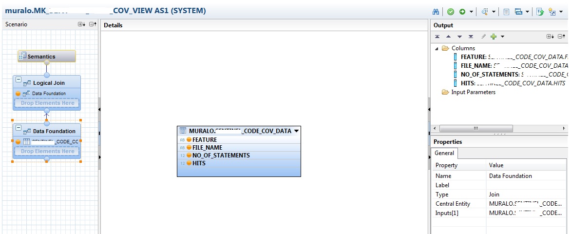
Click the Logical Join and Create Calculated Columns which are required in our case.

Let’s see the definition of each of these calculated columns

MISS and PERCENTAGE are not required, just ignore them.

Go to Semantics node and assign the Attributes and Measures

Save and Activate the Analytic View and check the Data Preview

Now the View is ready and can be consumed in Design Studio. But before that for the ease of analysis, I would like to see the coverage as different value buckets.

Eg :      

            Below < 25 %

Between 25 to 50 %

Between 50 to 75 %

            Above 75 %

For this purpose, I created four Calculation views using Projection, covering each bucket and applied the filter in it. Below one shows the filtering of < 25 %

Consuming in Design Studio :

Create an ODBC connection to the HANA system through odbcad32.exe

Launch Design studio, Add a Data source by connecting to this HANA system and open the view

Click the Application and go to its Properties pane, add a Global Script variable. The reason for adding this variable is, we can pass this variable as URL parameter and filter the data based on calendar week while launching the application

Edit the Initial View of inserted Data Source as shown below

Similarly insert the Calculation Views also and set the Initial View as

Now in the Application->Properties->On Startup, write the following Script

Place the components in the canvas as shown below

The Title, Calendar Week filter drop down, Separate tiles for each feature to show the respective Code coverage, Four charts to show the four categories (buckets) of coverage

Place the background image for better look and feel

Assign each Calculation views to each of these charts

Now the four charts have to show the coverage of the underlying files in four buckets for a particular feature when the user click on it

For Eg, If the user clicks on the coverage value of second tile (DASHBOARD), the files having coverage in different range should be shown in the charts accordingly

To achieve this, we can write following script for the OnClick event of Text placed in the tile which shows the value

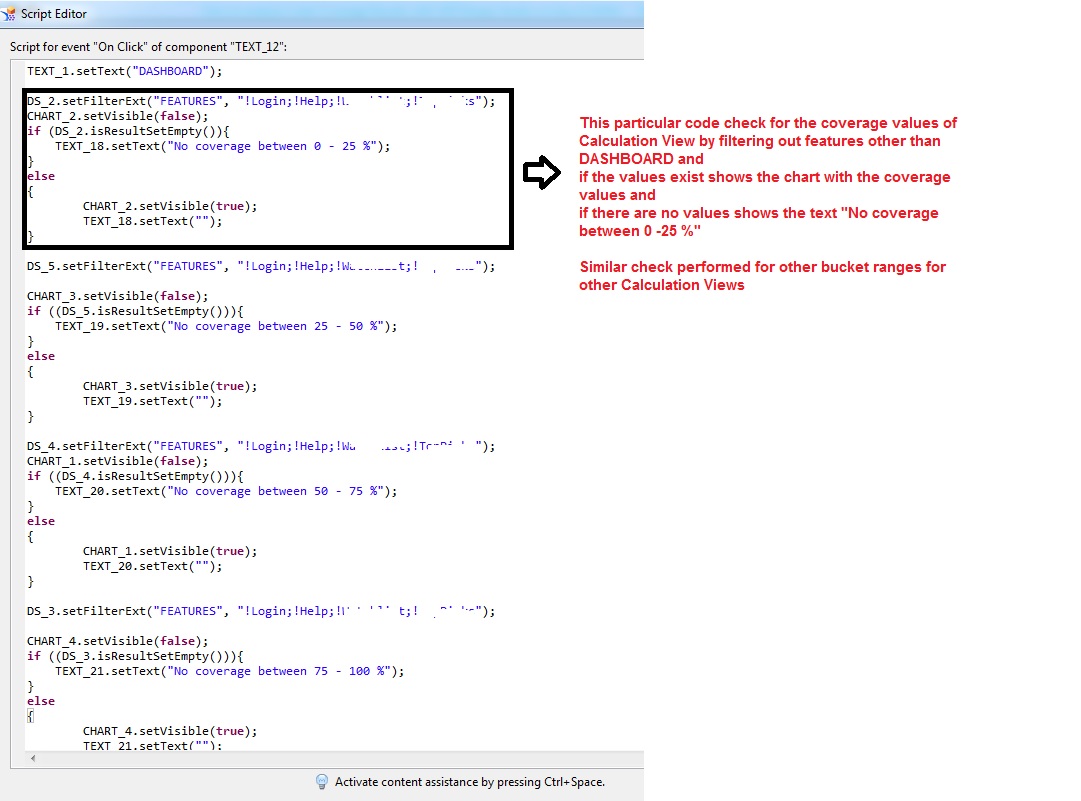
The same code can be copy pasted and changed accordingly for other Text placed in the tiles

Now Save the Dashboard and Execute

As mentioned earlier, here the Global Script variable value can be passed as URL parameter

“http://<server>:50130/aad/web.do?APPLICATION=<DashboardName>&Xcw=CW_06“

Here on clicking each tiles (DASHBOARD in this case), the respective coverage of Java Script(.js) files shown in each of the charts

On clicking HELP tile, there are no files with the coverage in the range of 0 – 25 % and 50 – 75 %

So if the user wants to find the list files covered < 50 % in each feature then he can focus more on Charts 1 and 2 which can show the files having coverage 0 – 25 % and 25 – 50 % and optimize the code.

Thanks for spending time in reading my article and Hope you find this helpful 🙂

Thanks & regards,

Murali